Example 02: Upward flow in a tank

Purpose

To calculate the density currents in an upward flow originated from a tank bottom. A low density boundary which has a lesser density than the background density generates this flow in a tank.

Creation of calculation grid and setting initial conditions

Create the calculation grid using [Grid] [Select Algorithm to Create Grid]. Then select Grid Creation Algorithem window will appear and then select [Gird Generator for Nays3DV] in select grid creating algorithm window.

Then grid creation window will appear. Select channel shape as shown in Figure 32.

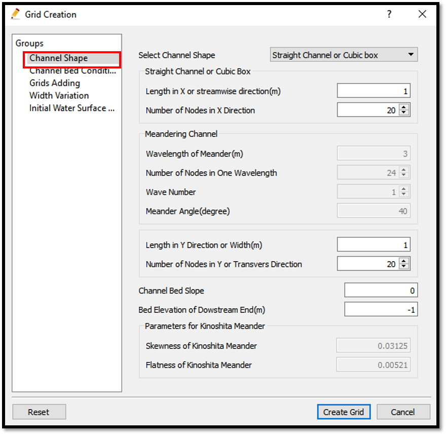
Figure 32 : Grid creation : Computational domain

Then we can give channel bed condition. As here we use the default condition flat(no bar) no modifications are needed.

If new grids are added or width is varied it is possible to set them. As in this example no grids added and no width variations, no modifications are needed in them.

Initial water surface profile tab is used to give downstream depth, water surface slope and initial water surface purtavation. It can be seen as shown in Figure 33.

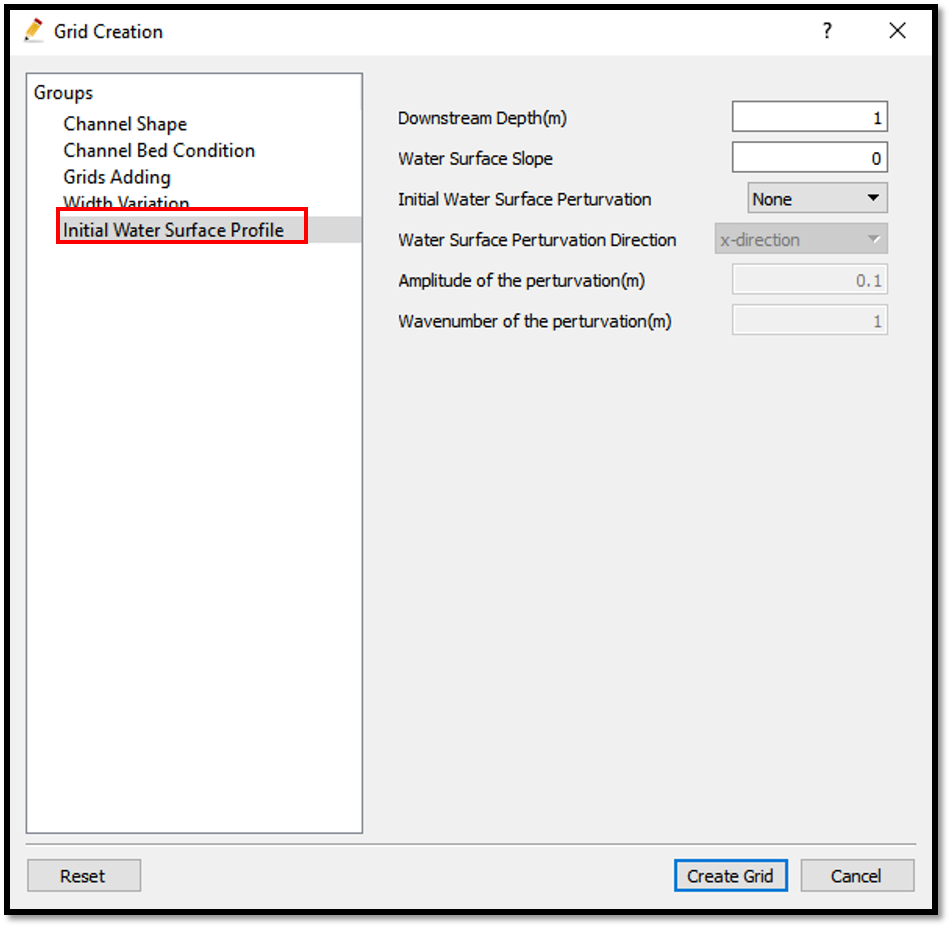
Figure 33 : Grid creation : Initial water surface profile

Here a tank is selected with a flat bed. After giving all the parameters as given in figures, select [Create grid]. Here a confirmation dialogue box will appear to map geographic data to grid attributes. Select yes and it will map the geographic data to the created grid.

The grid will be created as shown in Figure 34.

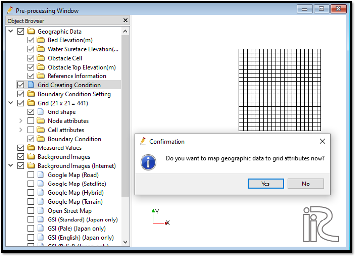
Figure 34 : Grid creation : Created Grid

Then by selecting node attributes and bed elevation in object browser, [Object Browser] - [Grid] - [Node attributes] - [Bed Elevation (m)], it is possible to see the geographic data mapped grid as shown in Figure 35.

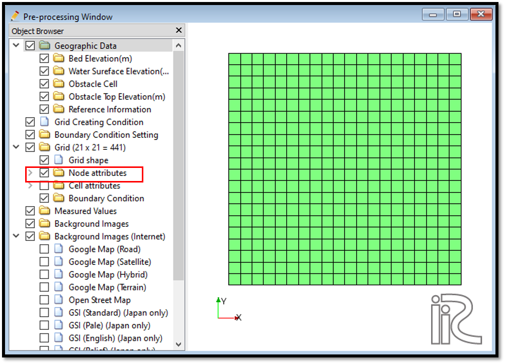
Figure 35 : Grid creation : Created Grid after mapping geographic data

It is always safer to see the attributes after mapping.

Now save the project with [File] [Save project as .ipro].

Setting the calculation conditions and simulation

Give the calculation conditions with, [Calculation Condition] [Settings].

Calculation cndition window will appear. Give computational parameters as shown in Figure 36.

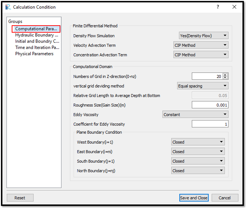
Figure 36 : Calculation_condition : Computational parameters

Now give the [Hydraulic Boundary Conditions]. Since the boundary conditions for this simulation were given as closed boundaries in computational parameters, hydraulic boundary conditions window is inactive in this example as shown in Figure 37.

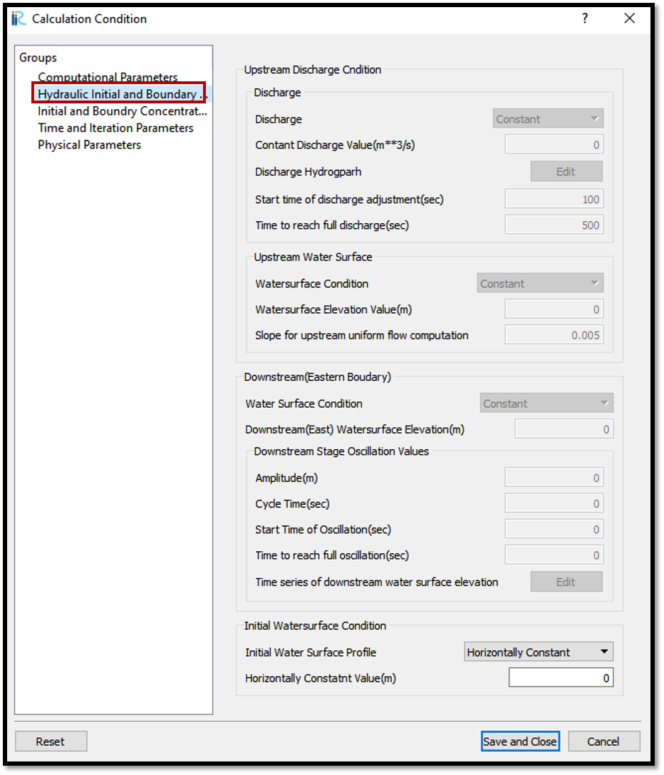
Figure 37 : Calculation_condition : Hydraulic Boundary Conditions

Now give [Initial and Boundary Concentration] as shown in Figure 38.

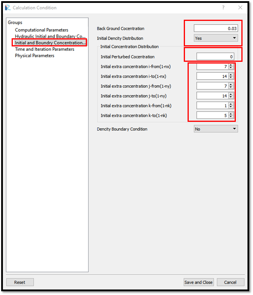
Figure 38 : Calculation_condition : Initial and Boundary Concentration

Here background concentration is the concentration in the tank and purturbed concentration is concentration of the down object which we create. In an upflow it is necessary to give initial purturbed concentration a lower value than the background concentration. Otherwise the upward flow won’t occur.

In the initial concentration distribution it is necessary to select the area of new concentration in all the directions i, j, k start and end grids.

Give time and iteration parameters as shown in Figure 39.

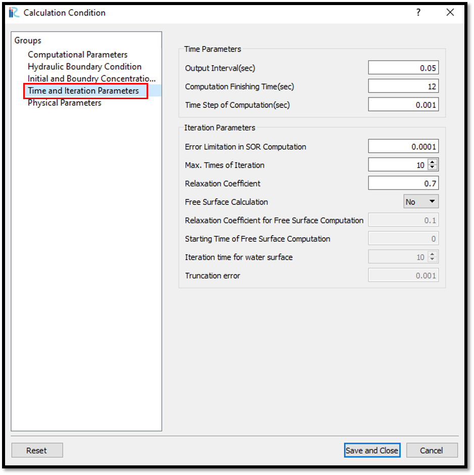
Figure 39 : Calculation_condition : Time and iteration parameters

Give physical parameters as shown in Figure 40.

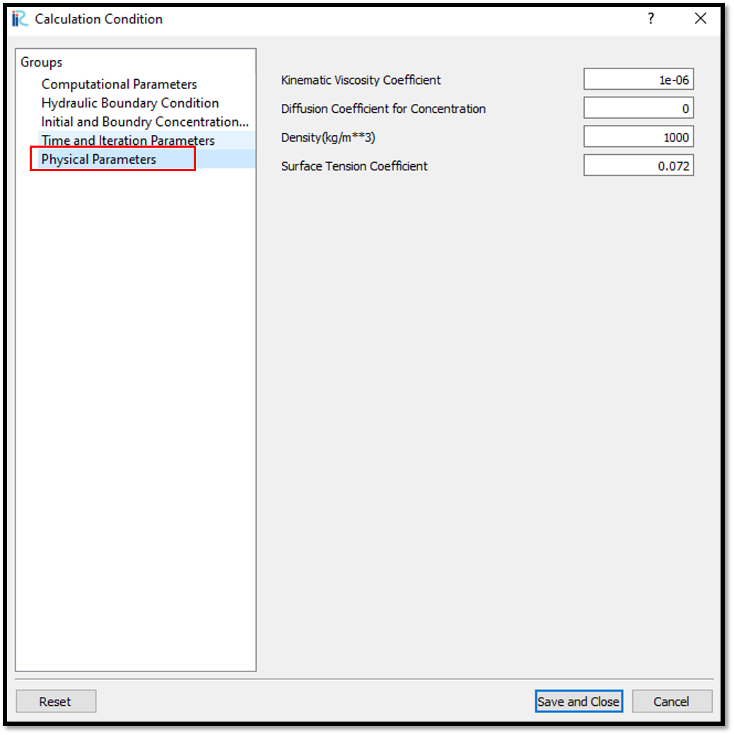
Figure 40 : Calculation_condition : Physical parameters

After setting the calculation conditions, save the project by clicking on save tab. Now start simulation by, [Simulation] [Run]. Simulation will start and after some time it will finish showing the message the solver finished the calculation.

Visualization of results

Open 3D post processing window by selecting, [Calculation Results] [Open new 3D Post-Processing Window].

Select any parameter in [Object Browser], [iRIC Zone].

In this example isosurface is selected as shown in Figure 41. When [Object Browser] - [Isosurface] - [Add] is selected, we can add isosurface of any parameter such as concentration, pressure, position, eddy viscosity, velocity etc. In this example concentration is selected.

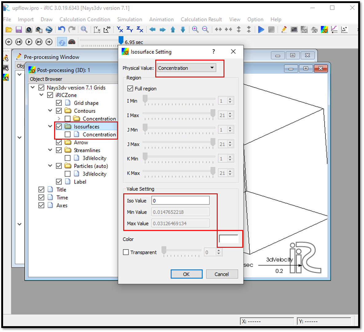
Figure 41 : Visualization of results : isosurfaces

In isosurface setting window, it is necessary to set physical value such as concentration, pressure, velosity etc which we need to plot. In value setting , we can see min value and max value as shown in Figure 42. Depending on our requirement we can select a value in between that min and max value.

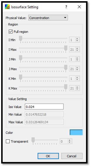
Figure 42 : Isosurface setting

Then we can select the colour for the isosurface as shown in Figure 43.

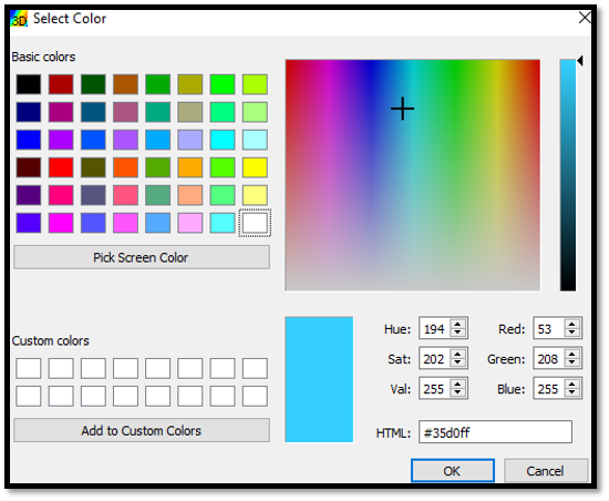
Figure 43 : Colour setting

Then we can see the isosurface of concentration as shown in Figure 44.

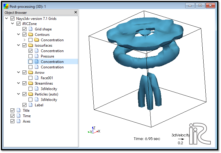
Figure 44 : Visualization of results : isosurfaces

Initial and final isosurfaces can be seen as shown in Figure 45.

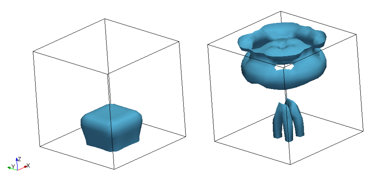
Figure 45 : Isosurface concentration

We can add arrows or contours to the plot as required.

To plot a concentration contour plot, go to [Object Browser] - [Contours] - right click at contours [Add]. Then contour setting window will appear as shown in Figure 46.

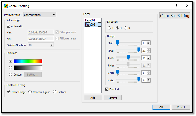
Figure 46 : contour setting : concentration

Here it is neccesary to add faces we nee to plot concentration. We can adjust the locations we need to plot by selecting region.

Figure 47 shows the concentration plot of the Zx plane.

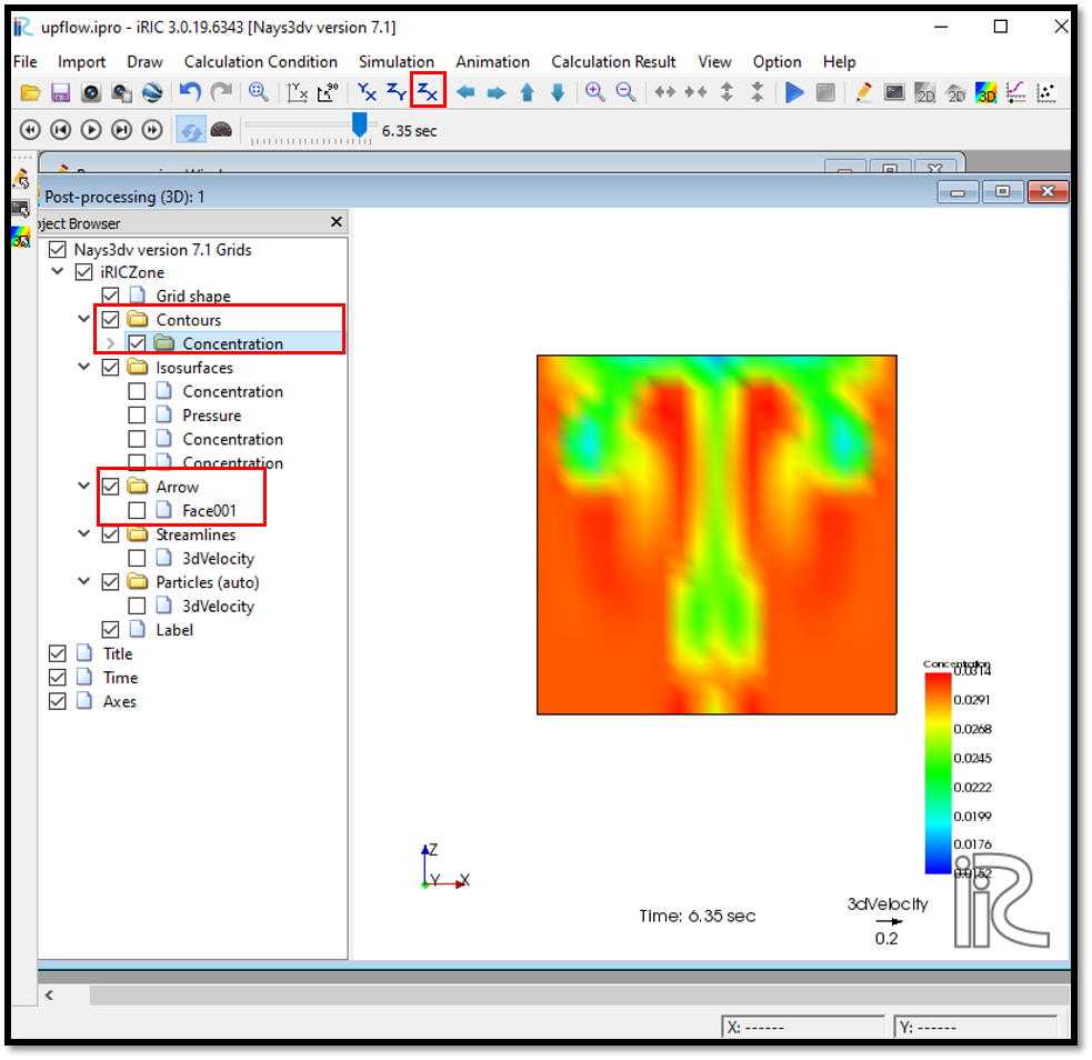
Figure 47 : contour setting : concentration