[Example 2] Suspended Material Transport in a Simple Bed Flume

In this section, we perform the following computations using a simple curved flume with straight inlet out let parts. The Cross section of the flume is composed with a compound channel in which both the low water channel and the flood plane with moveable bed. Then flood plane is located only left side of the low water channel. The experiment was carried out by CTI Engineering Co. Ltd. on behalf of Civil Engineering Research Institute of Cold Region . A movie taken from a drone during the experiment is shown in Figure 51, and the experimental condition and plane and cross sectional view pictures are shown in Figure 52.

Figure 51 : Experimental Video

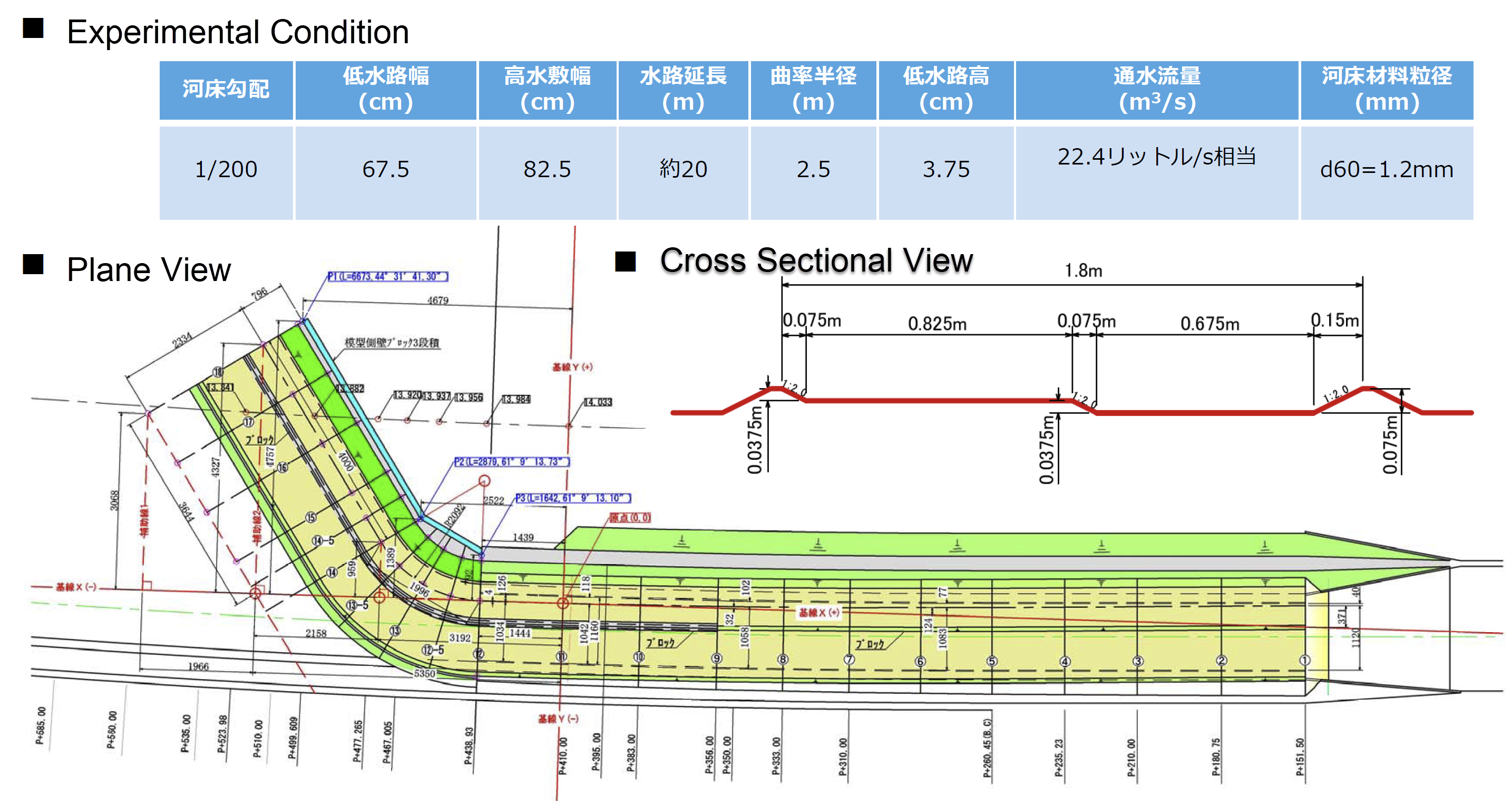
Figure 52 : Flume Shape

The computational exercises in this section is conducted as the following procedure.

• Flow and bed deformation by Nays2DH until the bed reaches an equilibrium state

• Quasi 3-dimensional flow field by Nays2d+

• Tracer tracking by UTT．Check the effect of turbulent diffusivity by changing parameter

Calculation of Flow and bed deformation by Nasy2DH

Select a Solver

From the iRIC startup screen, click [Create New Project], and select [Nays2dH iRIC3x 1.0 64bit] in the Figure 53.

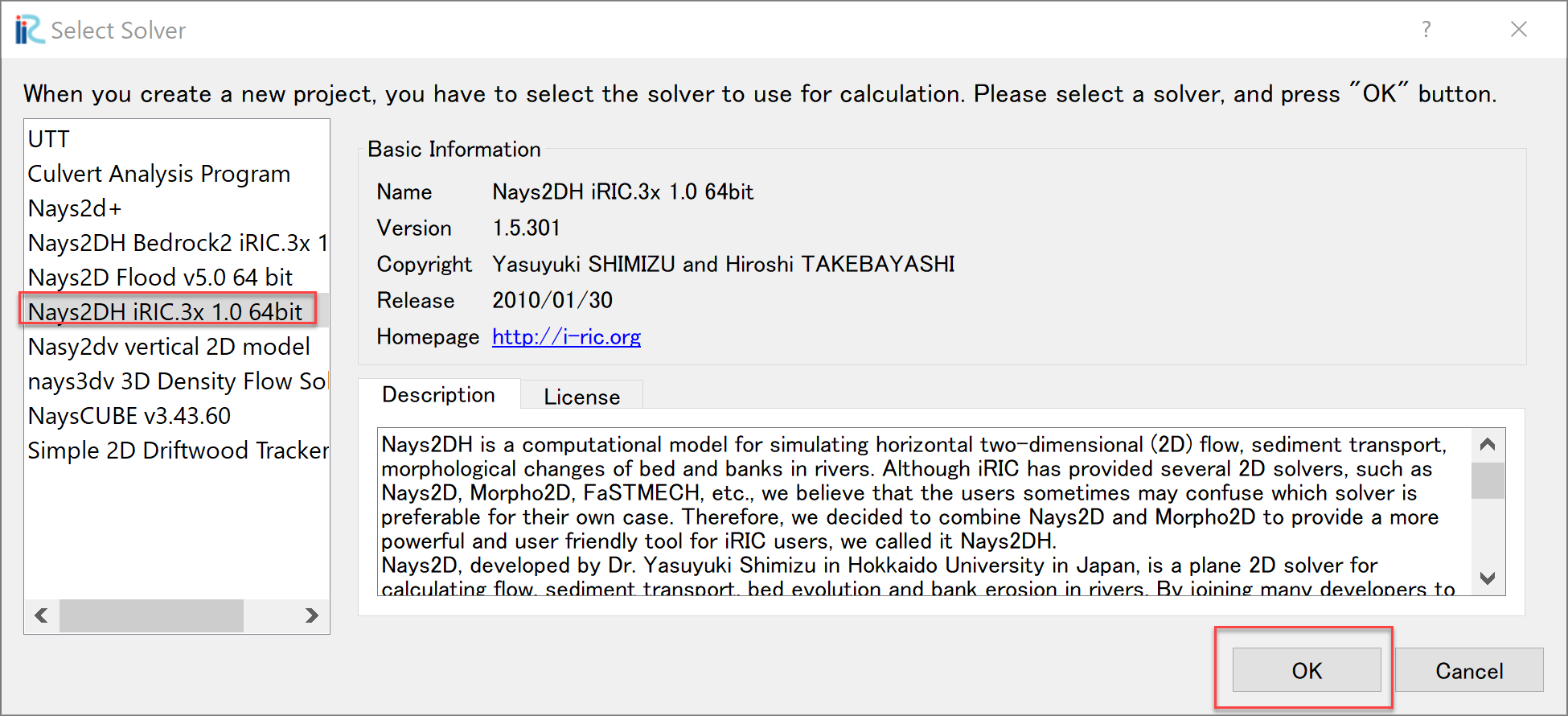
Figure 53 : Solver Selection

A window titled as「Untitled- iRIC 3.x.xxxx [Nays2DH iRIC3X 1.0 64bit]」appears.

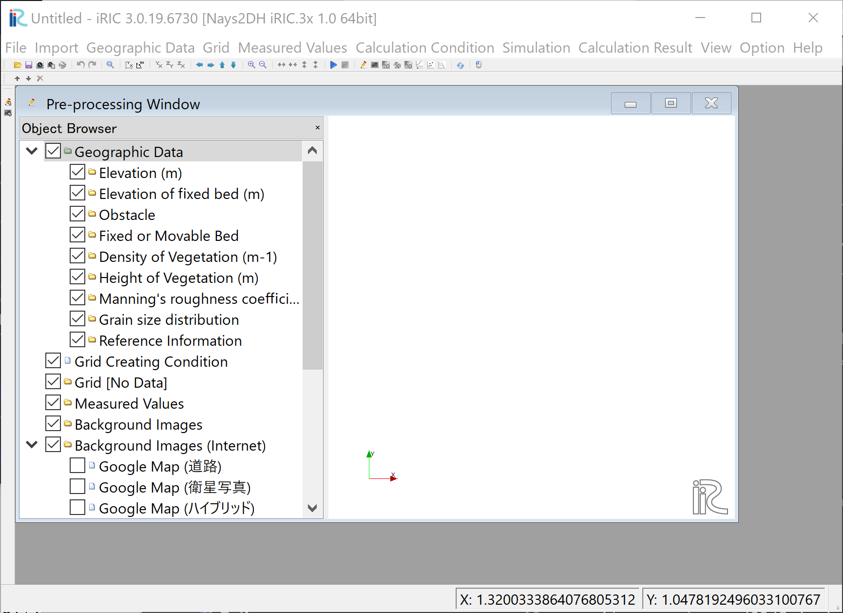
Figure 54 : Launch Nays2DH

Grid Creation

Select from the main menu [Grid]->[Select Algorithm]. Then a window appears as Figure 55, select [2d arc grid generator (Compound Channel)] and click [OK].

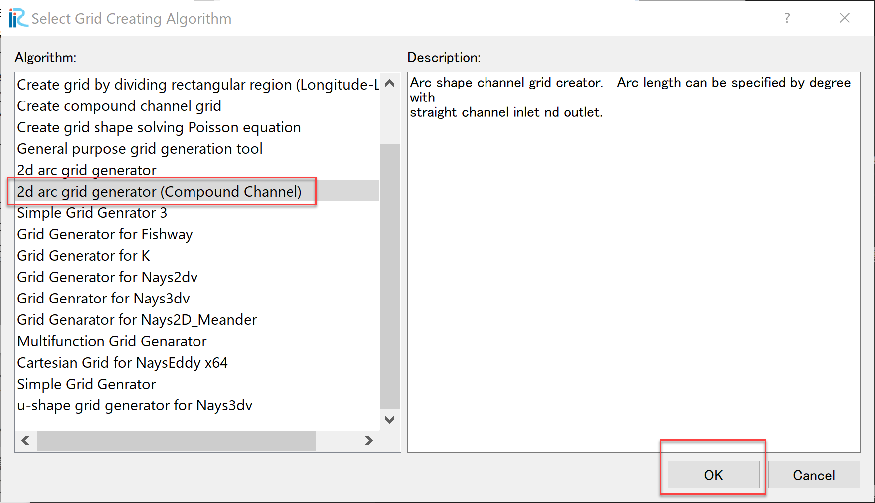
Figure 55 : Select Algorithm to Create Computational Grid

In the [Groups] of the [Grid Creation] window, set parameters of, [Channel shape], [Cross section], [Additional Channel] and [Roughness and fixed/moveable bed] as, Figure 56 , Figure 57 , Figure 58 , and Figure 59 , respectively.

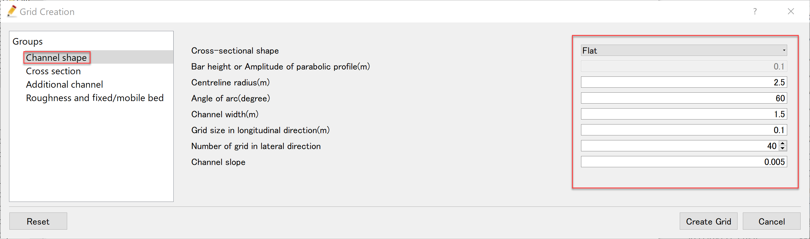
Figure 56 : Grid Creating Condition(1)

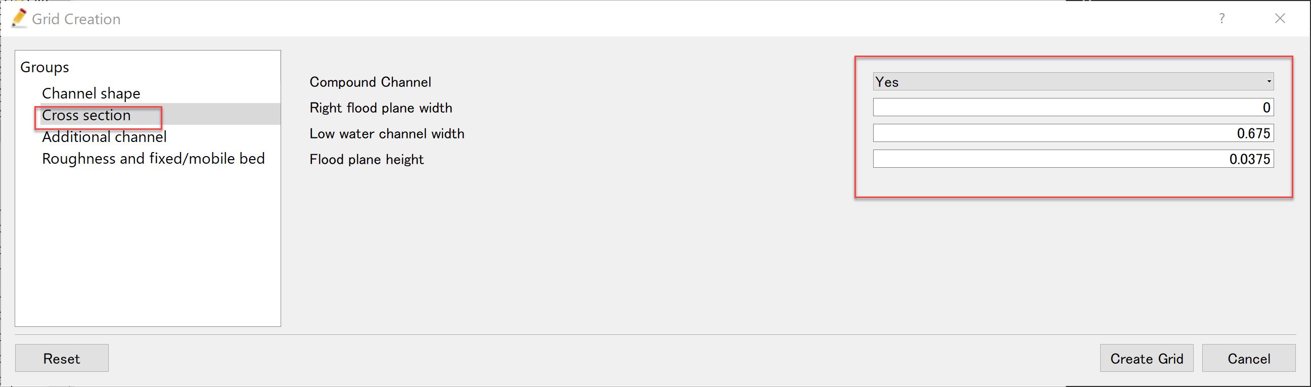
Figure 57 : Grid Creating Condition(2)

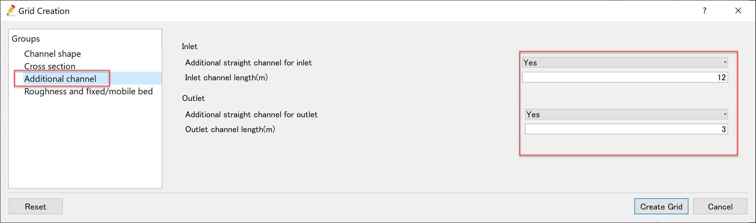
Figure 58 : Grid Creating Condition(3)

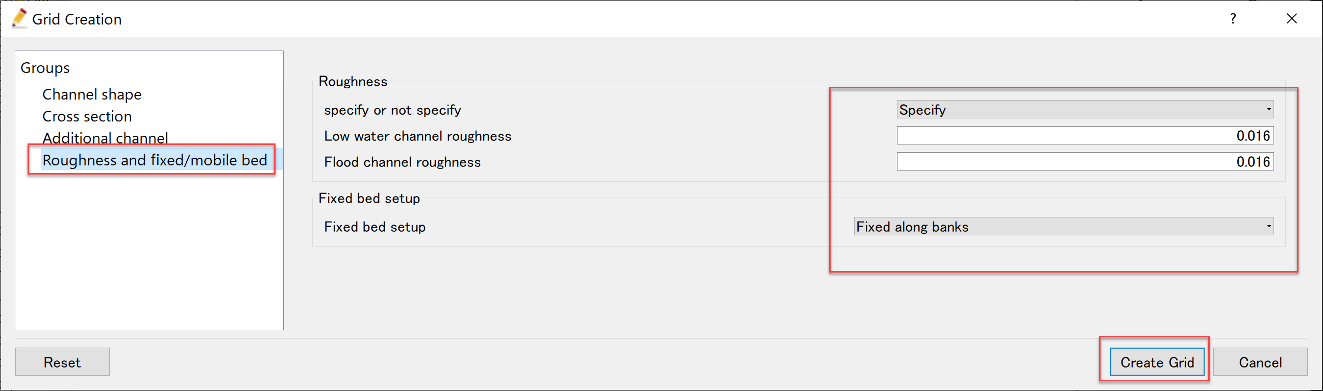
Figure 59 : Grid creating Condition(4)

When you finished all the settings of the grid creating condition, click [Create Grid] in the above grid creating condition windows, e.g. Figure 59. After clicking [Create Grid] button, you will be asked [Do you want to map?], then answer [Yes], and the computational grid is created. ( Figure 60 )

Figure 60 : Confirmation of mapping.

Put check marks in [Grid], [Cell Attributes] and [Fixed or Moveable bed] in the object browser, Figure 61 appears with the fixed bed part in red and the moveable bed part shown in blue.

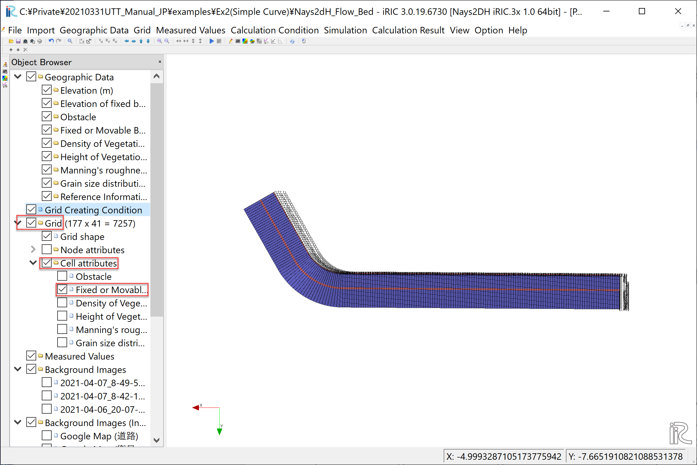
Figure 61 : Grid Shape with Fixed and Moveable bed Colored

The red part of the fixed bed along the boundary between the low water channel and the flood plane is assumed to be a revetment, in this grid creating tool, however, since the revetment in the actual experiment is only the bend part plus short length of upstream and downstream. So, as shown in Figure 62, focus [Fixed or Moveable bed], and right-click on a straight section of the revetment part (in this case, the red section upstream of grid number 87) and change the attribute to [Moveable bed], and press [OK].

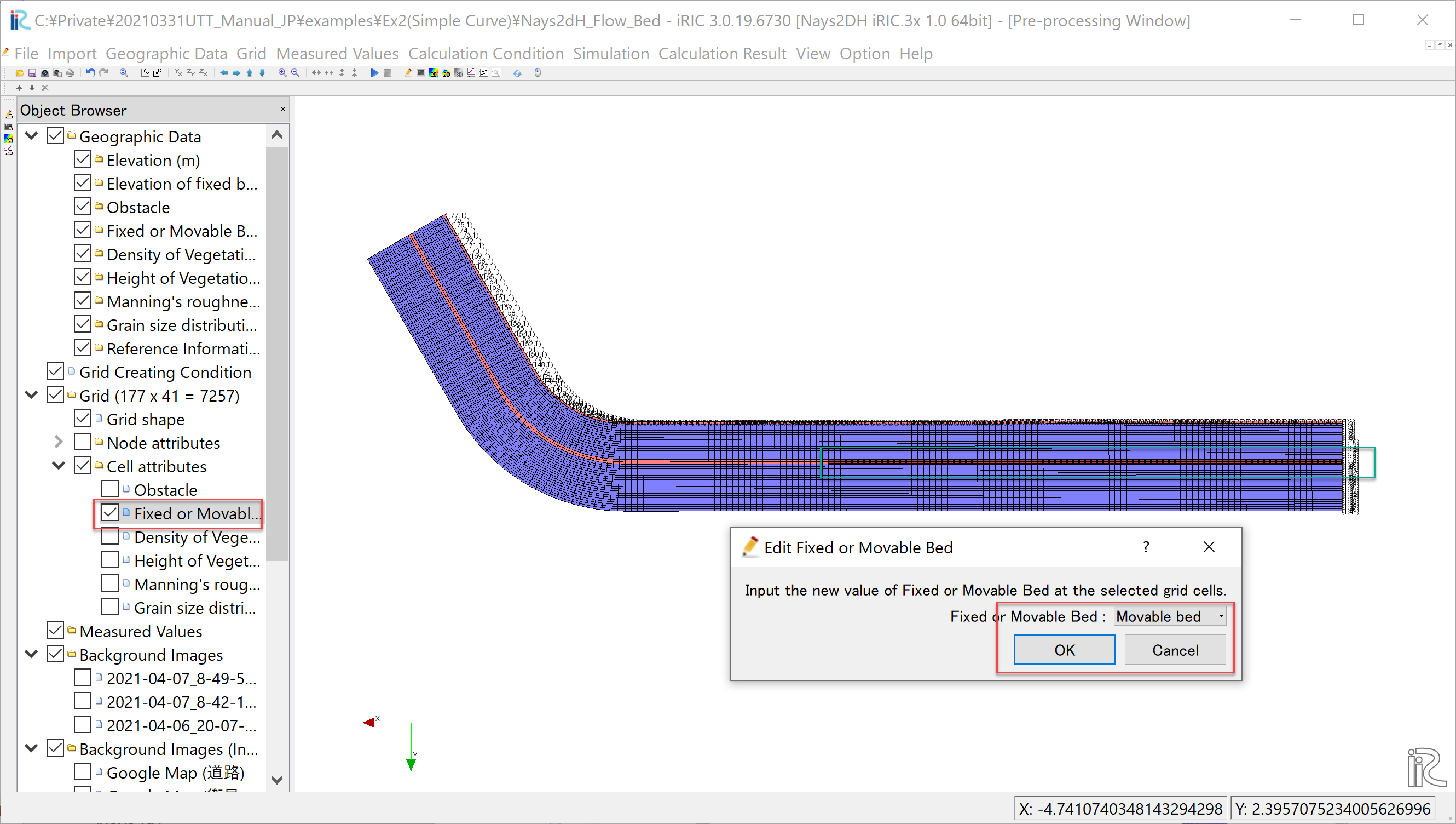
Figure 62 : Change attribute from fixed bed to moveable bed

Since the downstream end is the fixed bed, set the attribute of the downstream end cells into [Fixed Bed], by expanding and rotating, as demonstrated in Figure 63.

Figure 63 : Change downstream end cell attribute to fixed bed

Setting Computational Condition

Show the [Calculation Condition] window by selecting [Calculation Condition]->[Setting], and in the [Group] of [Solver Type], [Boundary Condition], [Time] and [Bed Material] , set the parameters, as Figure 64 , Figure 65 , Figure 66 , and Figure 67, respectively.

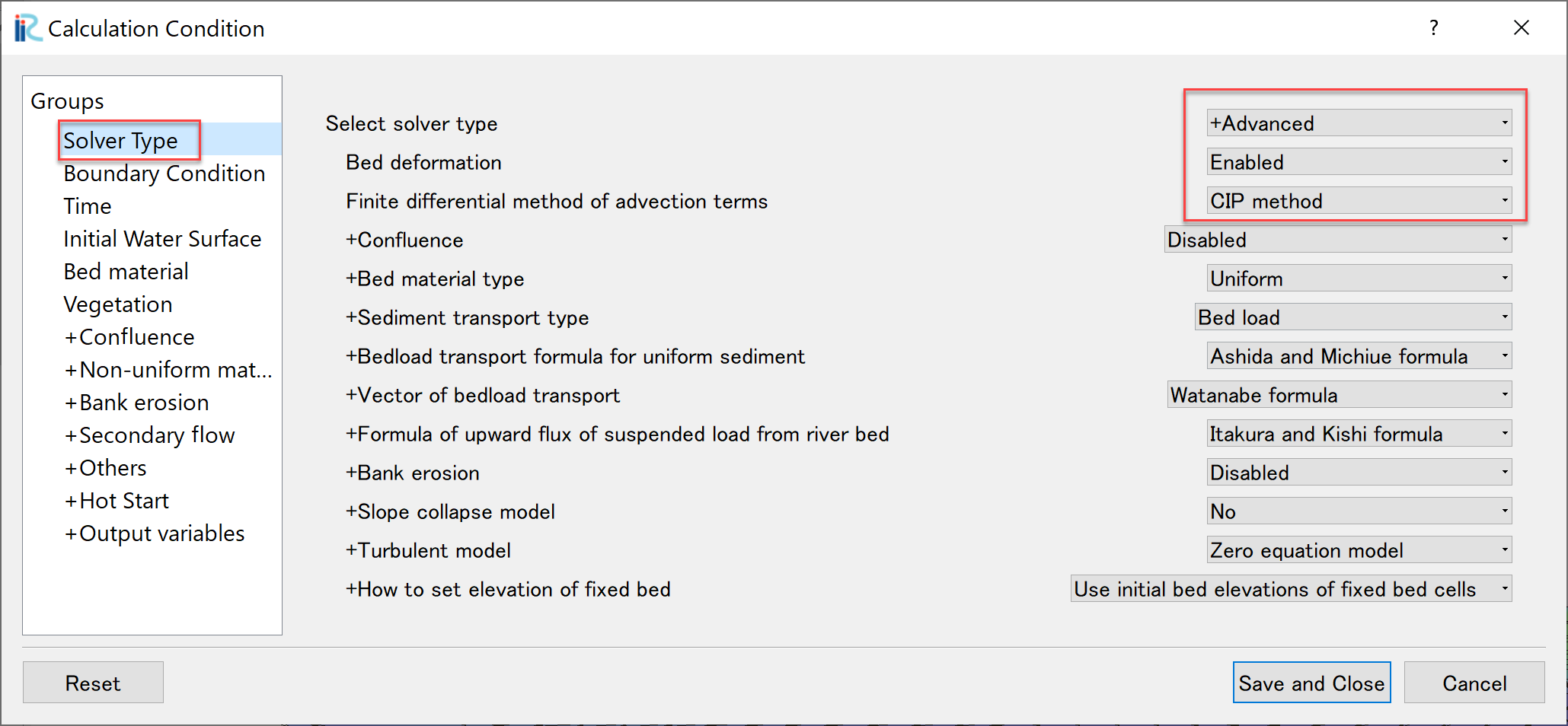
Figure 64 : Calculation Condition(Solver TYpe)

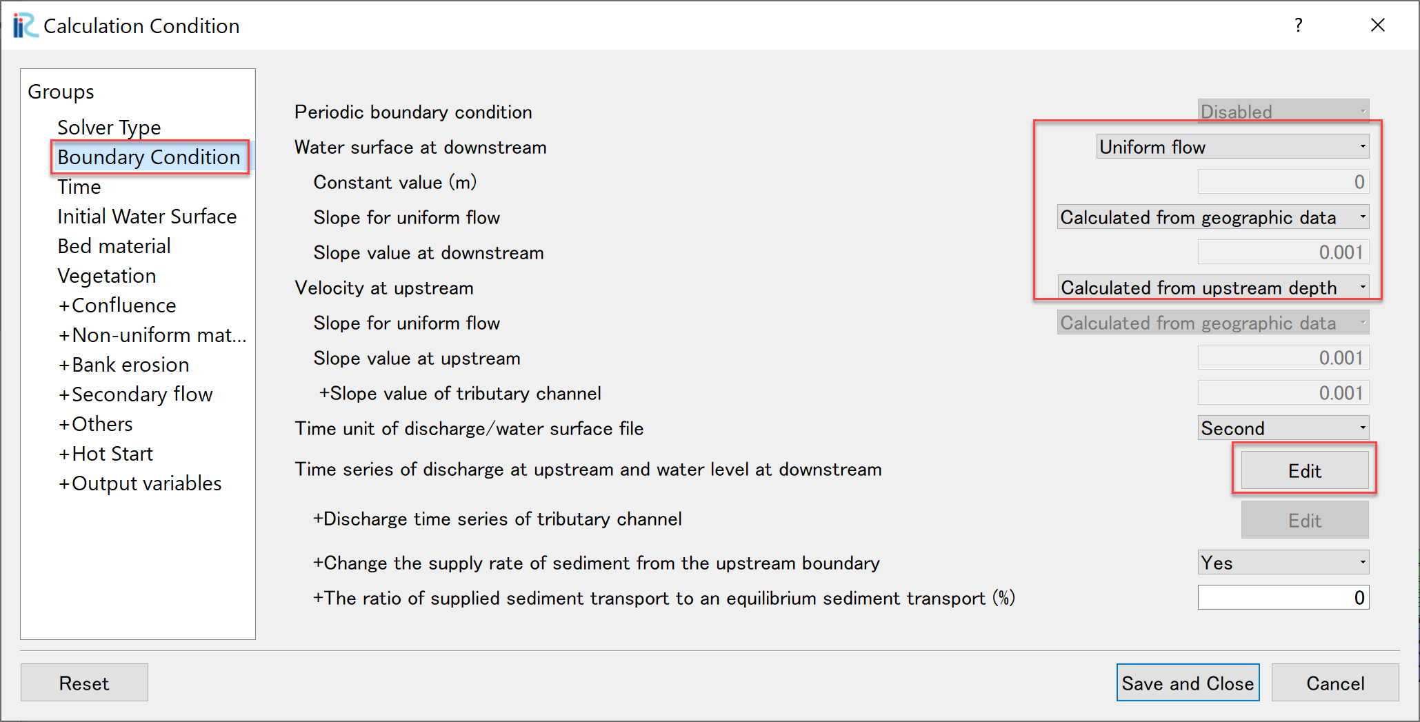
Figure 65 : Calculation Condition(Boundary Condition)

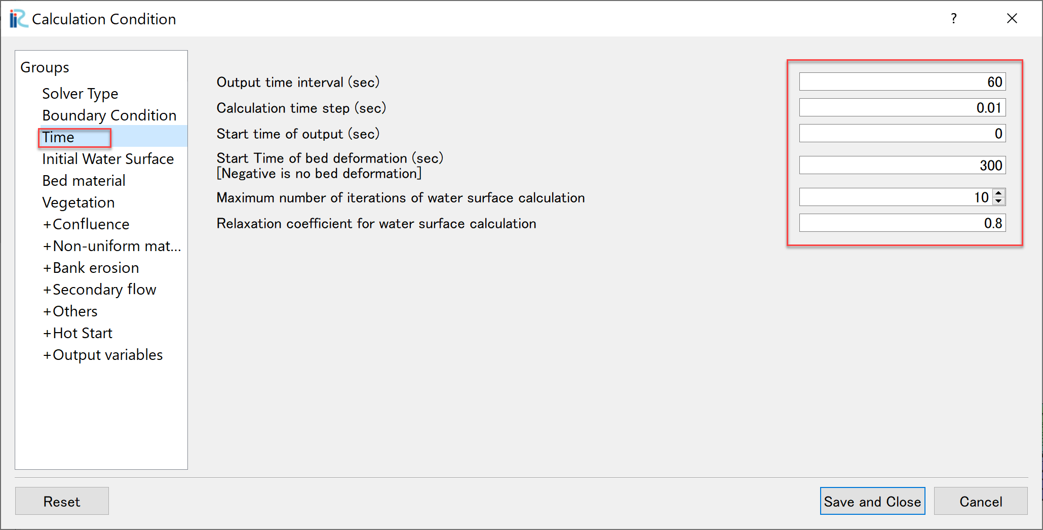
Figure 66 : Calculation Condition(Tme)

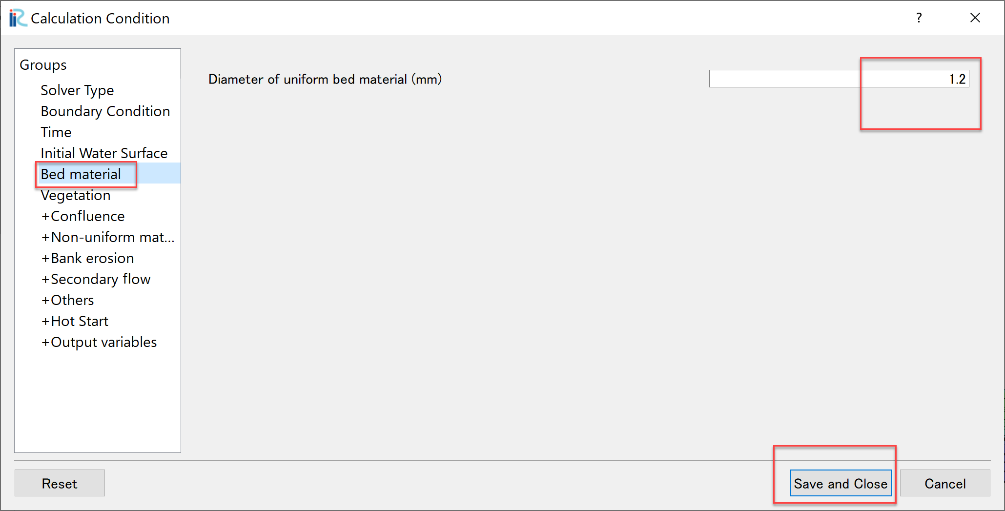
Figure 67 : Calculation Condition(Bed Material)

In addition, in the [Boundary Condition] setting of Figure 65, press [Edit] of [Time series of discharge at upstream end ……], and set [Time] and [Discharge] hydrograph data in the [Time series of discharge at upstream end ……] window as Figure 68, and press [OK].

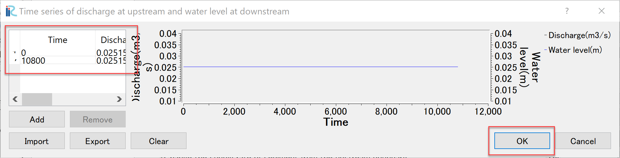
Figure 68 : Setting Discharge Hydrograph

When you finished the settings of all the computational condition parameters, press [Save and Close] in the [Calculation Condition] window.

Run Nays2DH

Before executing the Nays2DH, select [File]->[Save as Project] and save the project. Here we save the project as a name of [Nays2DH_flow_bed] (Figure 69)

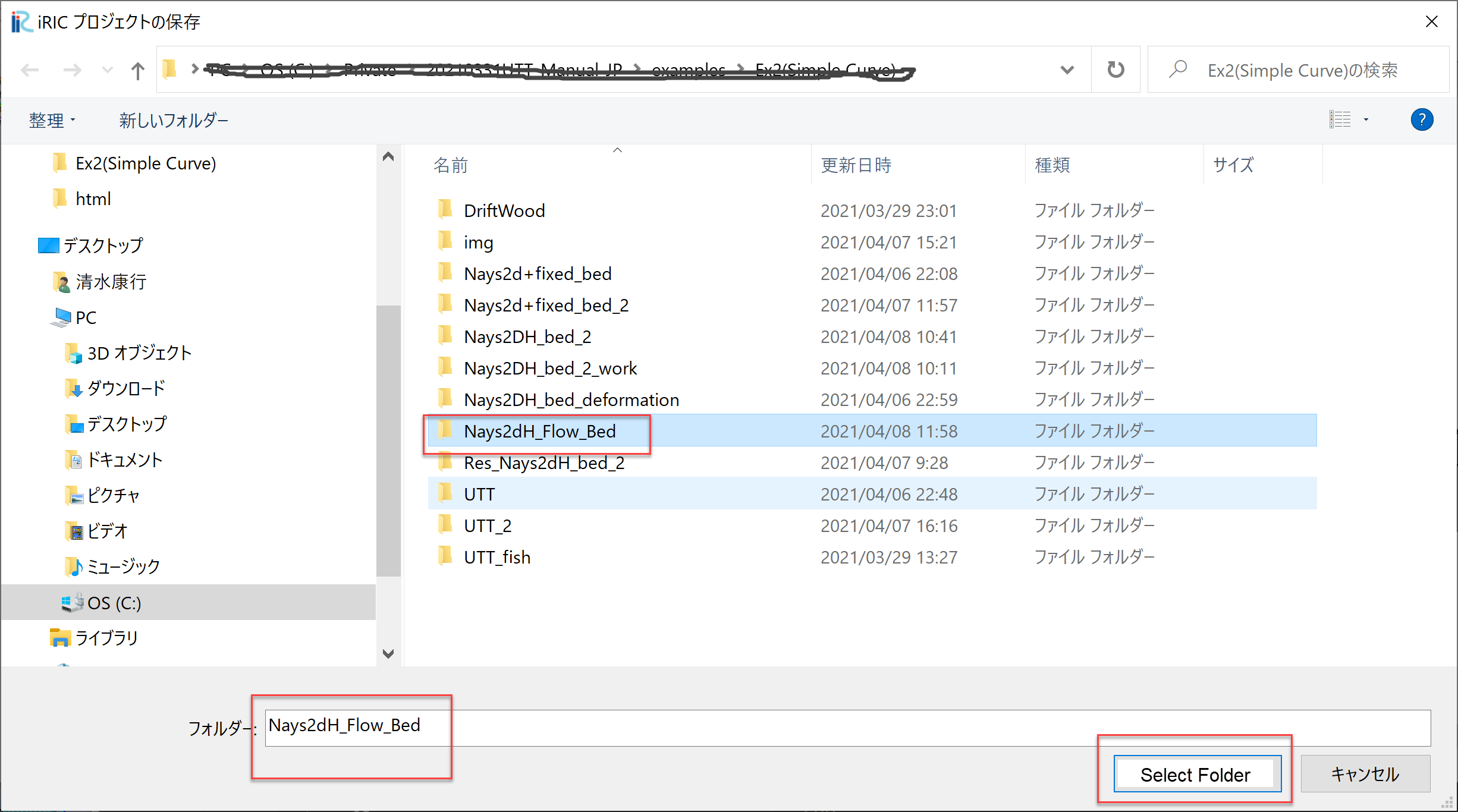
Figure 69 : Save Project

From the main menu, select [Simulation]->[Run], then a window asking [Do you want to save?] appears as Figure 70. Then press [Yes], save as a project, and the computation starts running as Figure 71.

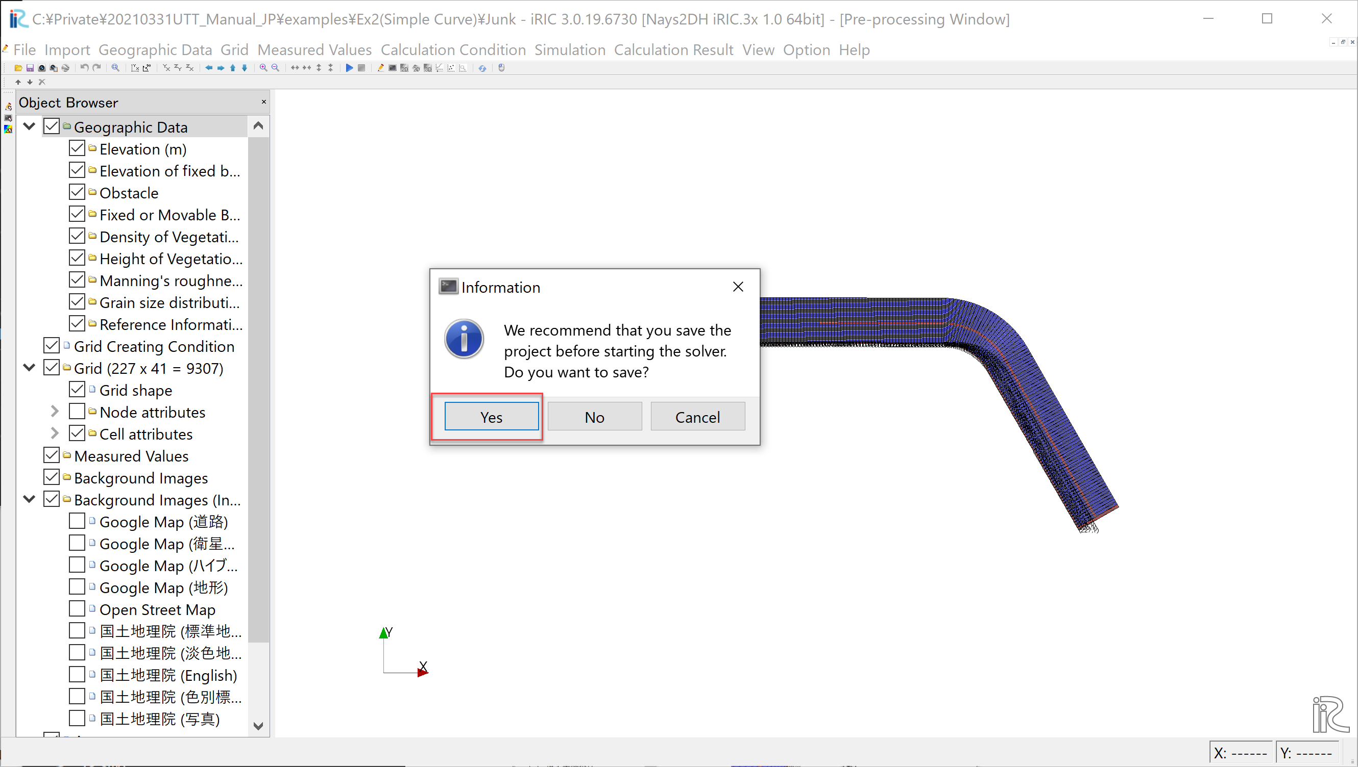
Figure 70 : 「Do you want to save?」

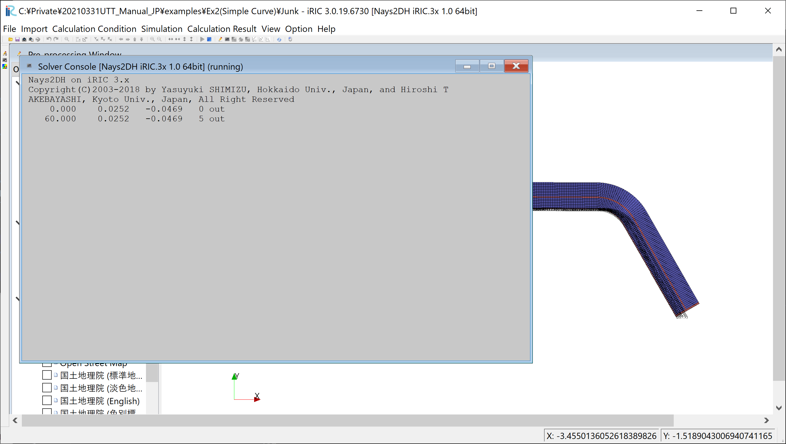
Figure 71 : 「Nays2dH is running」

When the computation finished, save the results by selecting [Calculation Result]->[Save], from the main menu.

Display the Calculation Results

Open a [Post Processing Window] by selecting [Calculation Result]->[Open new 2D Post-Processing Window] as Figure 72.

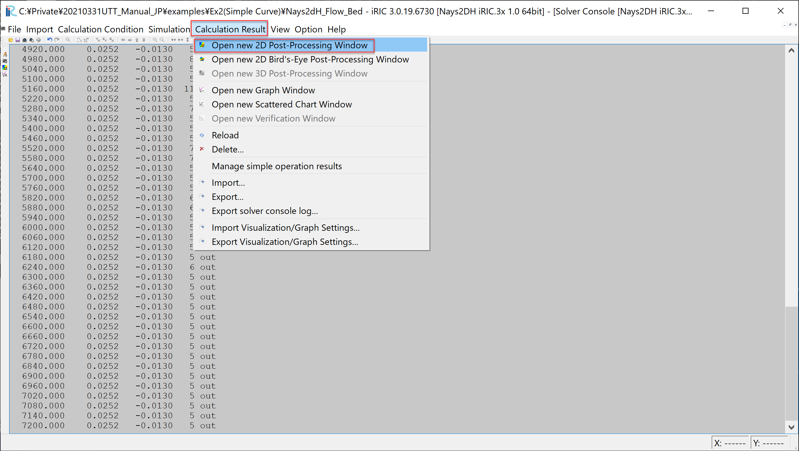
Figure 72 : Open Post Processing Window

In the object browser of the [Post Processing Window], put check marks in [iRICZone], [Scalar(node)] and [ElevationChange(m)]， right click [ElevationChange(m)] to show [Property] and press it, open [Scalar Settings], and set parameters as Figure 73.

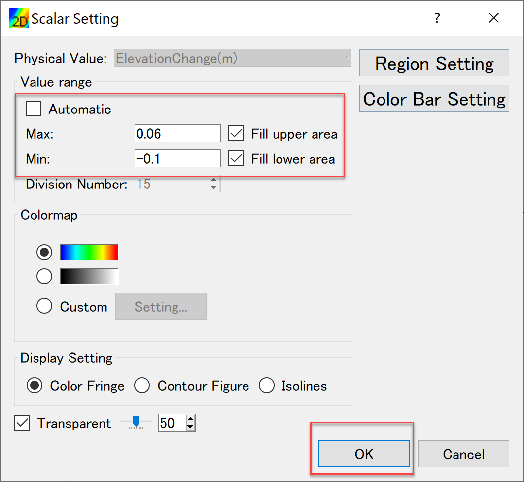
Figure 73 : 「Scalar Setting」

In the object browser, put check marks in [Arrow] and [Velocity(m)], right click [Arrow], show [Property] and press it, open [Arrow Setting Window] as Figure 74, and set parameters as marked with red squares in the Figure 74.

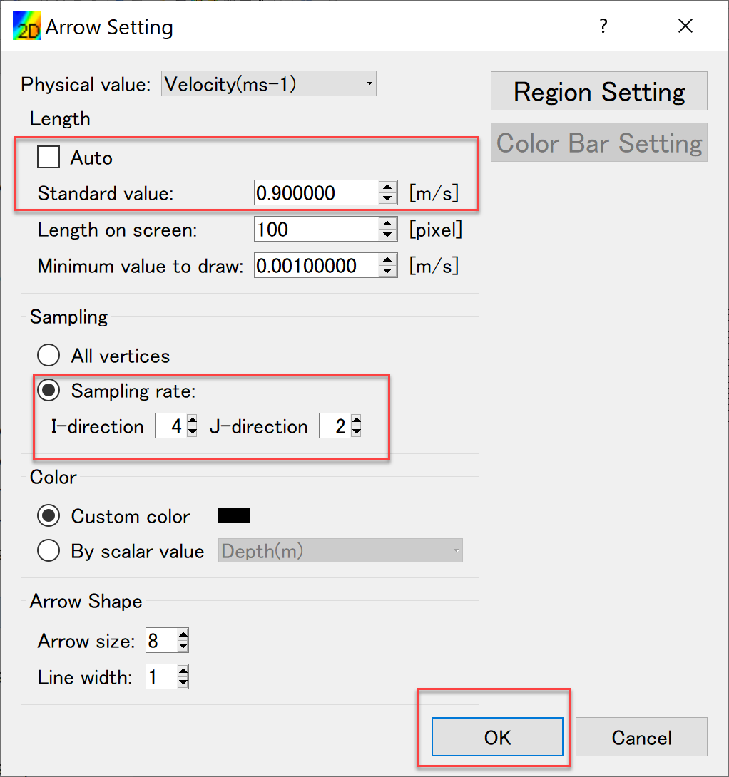
Figure 74 : [Arrow Settings]

Put the [Time Scale Bar] back to zero, select [Animation]->[Srart/Stop] to start animation as Figure 75.

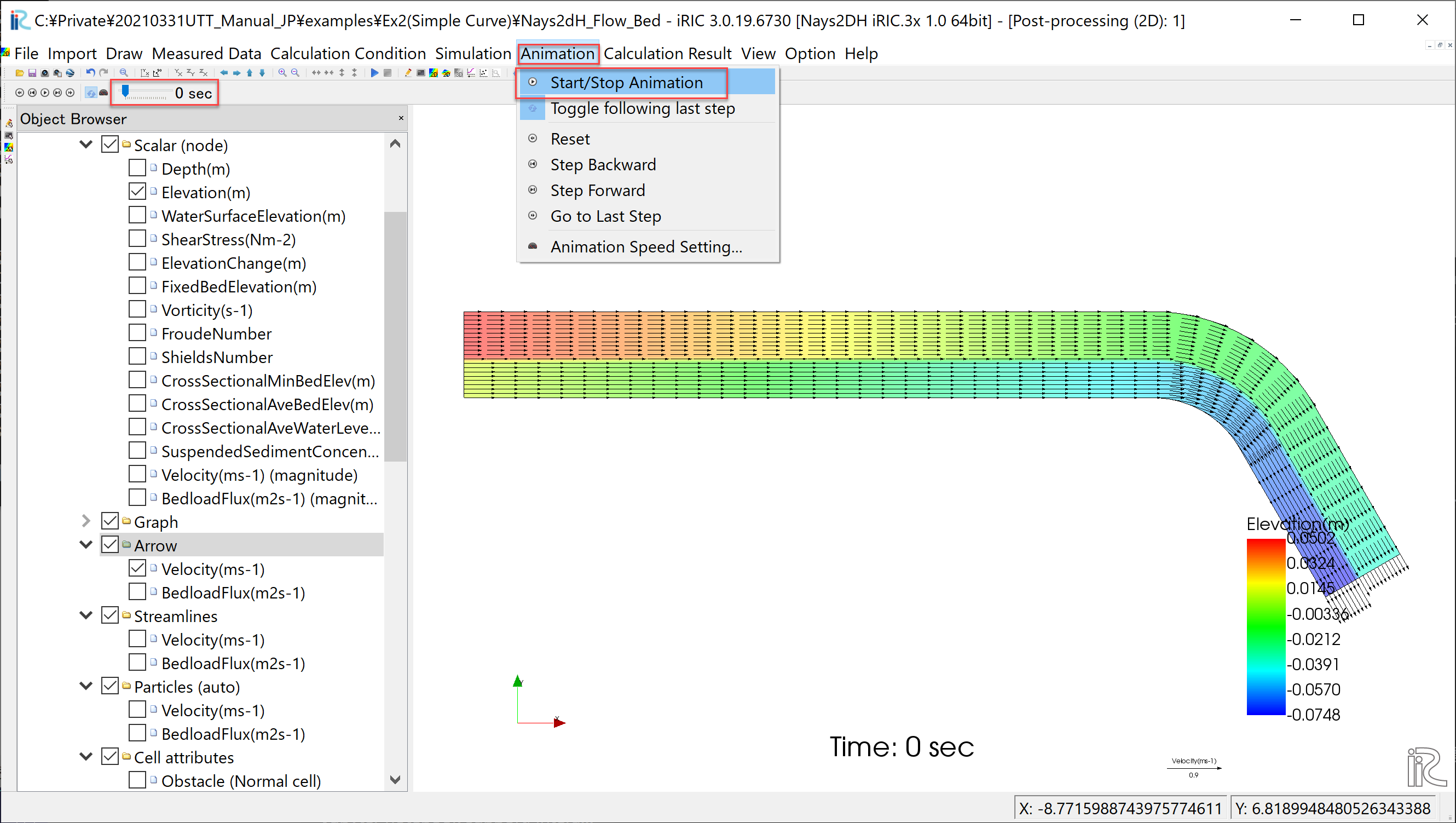
Figure 75 : [Launch Animation]

As shown in Figure 76, it is shown that the bed elevation change reached an equilibrium.

Figure 76 : Animation of velocity vectors and bed elevation changes

Export the Computational Results

In order to use the calculated bed elevation as an boundary conditions for the quasi-3D flow calculation by Nays2d+ in the next section, we export the calculated results to a text file. As shown in Figure 77, select [File]->[Export]->[Calculation Result].

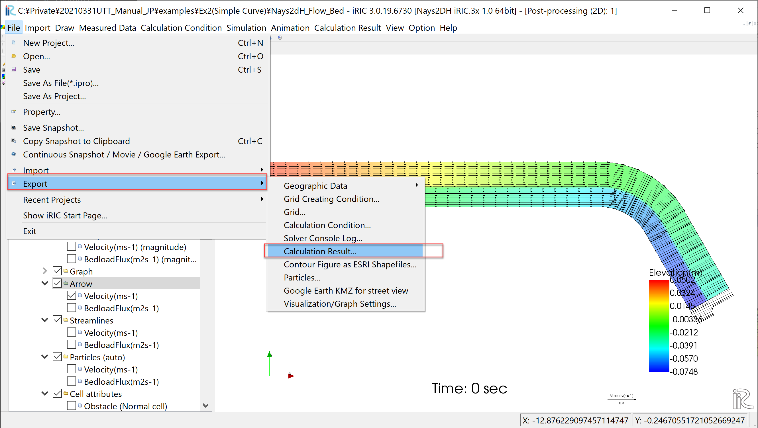
Figure 77 : Exporting Computational Results(1)

When the [Export Calculation Result] setting window (Figure 78) is appeared, choose [Format] as [Topography Files(*.tpo)].

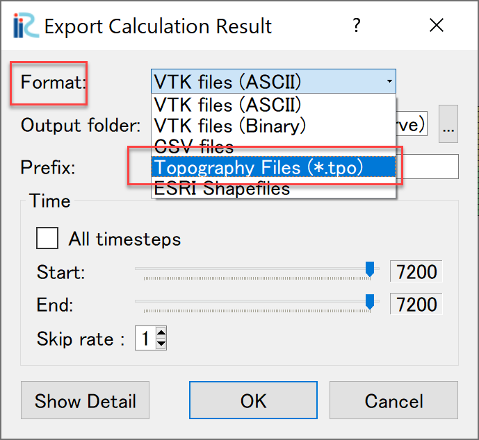
Figure 78 : Exporting Computational Results(2)

The output folder can be any name, and uncheck the checkbox at [All timesteps], and set [Start] and [End] as 7,200. Then click [OK] to complete the export of the calculation Results Figure 79．

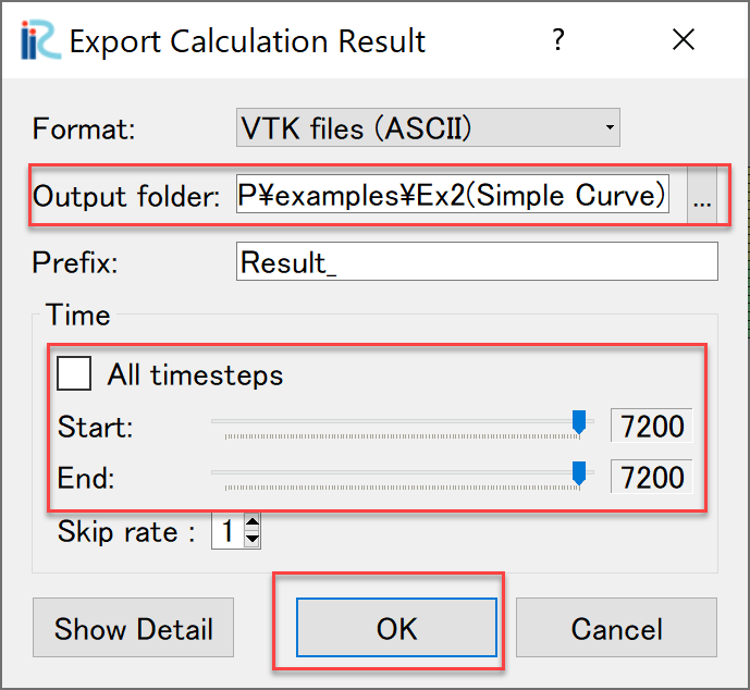
Figure 79 : Exporting Computational Results(3)

The exported calculation results are stored in the specified folder. As shown in Figure 80, many files contain different values as water depth, velocity, sediment transport rate, riverbed elevations, and so on, however, since only the riverbed elevation is used for the flow calculations in the next section, all files except [Result_1_Elevation(m).tpo] can be deleted.

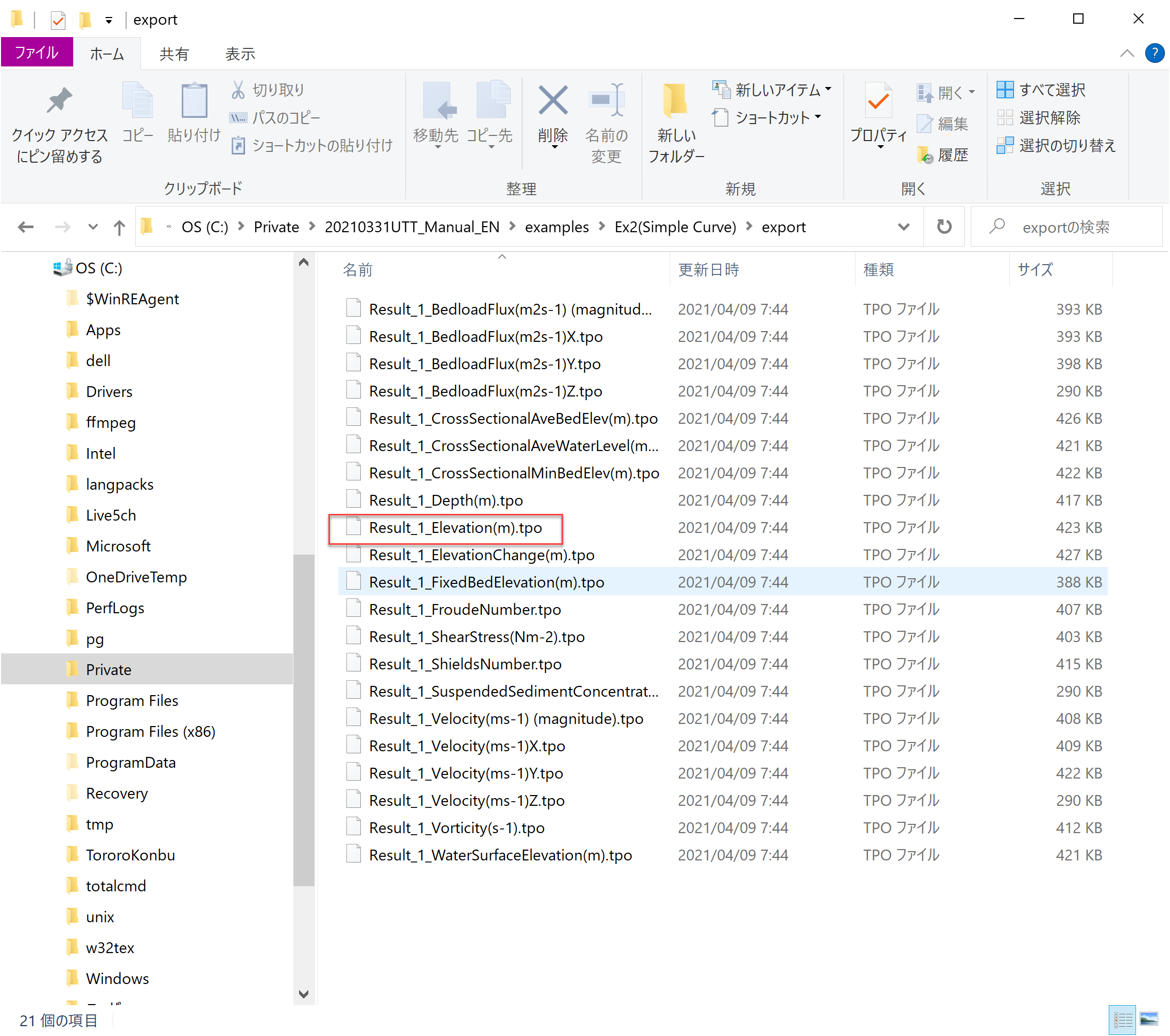
Figure 80 : Exporting Computational Results(4)

Quasi-3D Flow Calculation by Nays2d+

Selecting a Solver

From the iRIC startup screen, click [Create New Project], and select [Nays2d+] in the Figure 81, and press [OK].

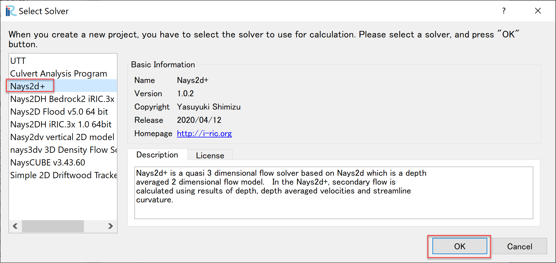
Figure 81 : Solver selection of Nays2d+

Importing Computational Grid, Channel Bed Elevation and Mapping

Importing Grid

From the main menu, select [Import]->[Grid], and choose [Case1.cgn] in the folder of [Nays2DH_floe_bed] which was created in the previous section. While importing, a warning as Figure 82 is coming out, press [Yes], and complete importing grid (Figure 83).

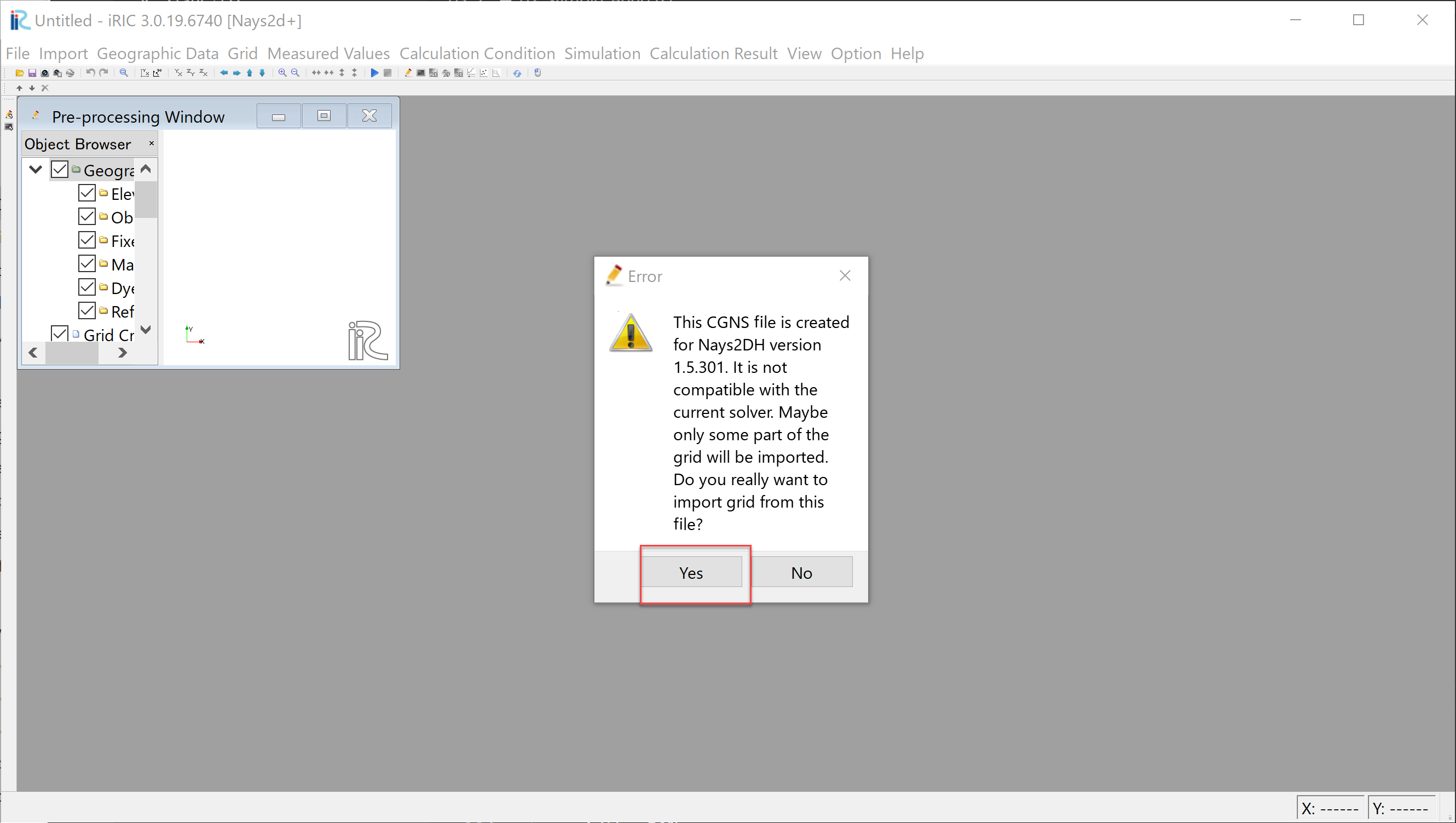
Figure 82 : [Warning]

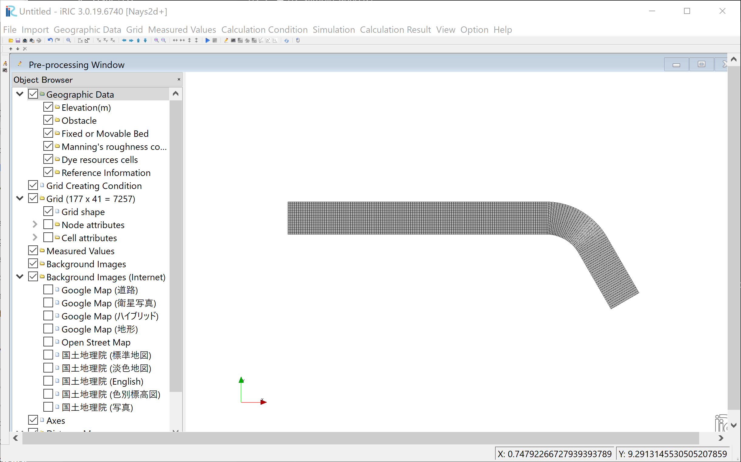
Figure 83 : [Grid import complete]

Import Bed Elevation

From the main menu, select [Import]->[Geographic Data]->[Elevation](Figure 84).

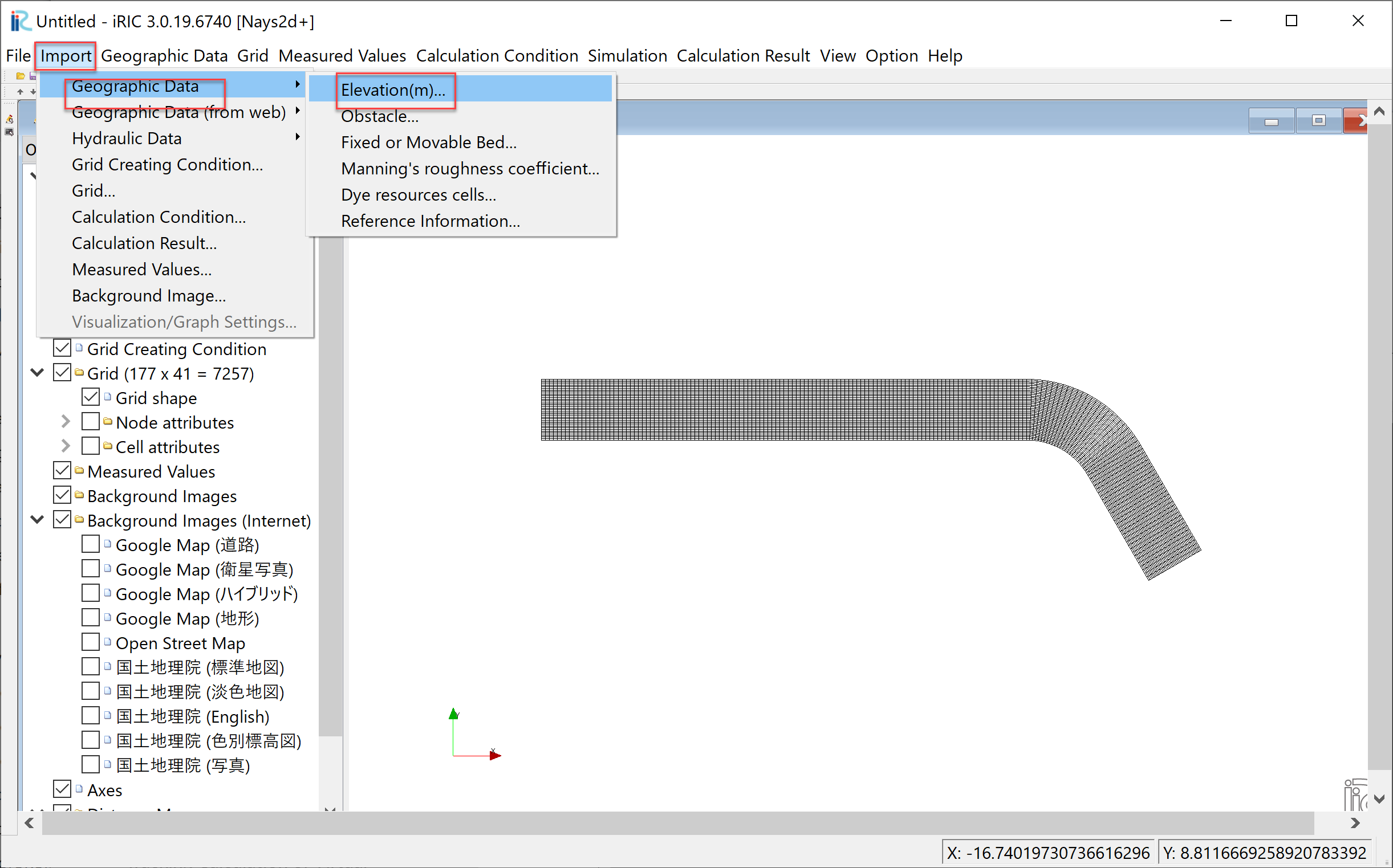
Figure 84 : Import Elevation

In the import file selection window, Figure 85, assign the file [Results_1_Elevation(m).tpo], which was exported from Nays2dH calculated results in the previous section.

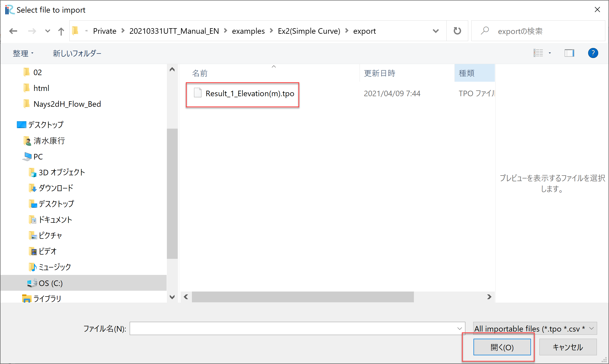
Figure 85 : Select bed elevation file to import

Figure 86 appears, but if there is no particular need to thin out the data, you can leave it as it is, and press [OK] to complete the import the [Bed Elevation] (Figure 87).

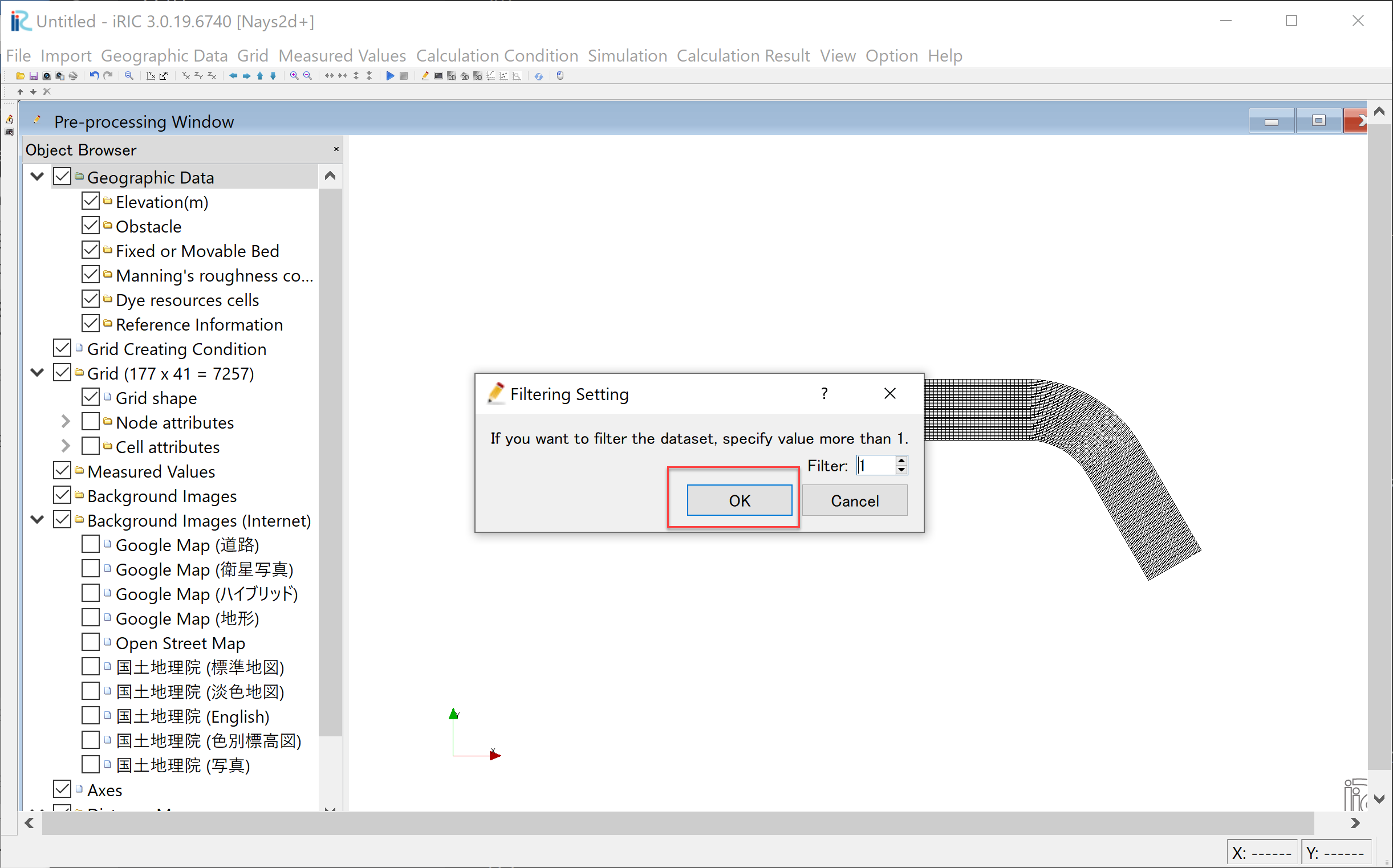
Figure 86 : Import Bed Elevation (Setting Thinning)

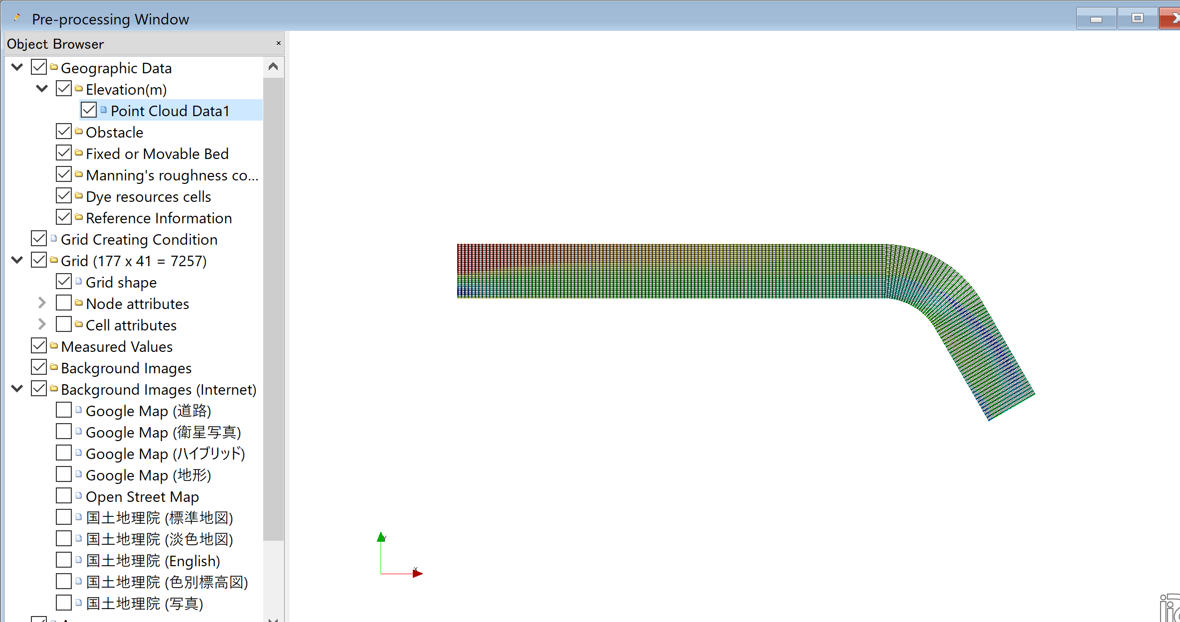
Figure 87 : Bed Elevation Data Import Completed

Execute Mapping

The imported bed elevation data is mapped onto the imported computational grid. Select [Grid]->[Attribute Mapping]->[Execute] as Figure 88.

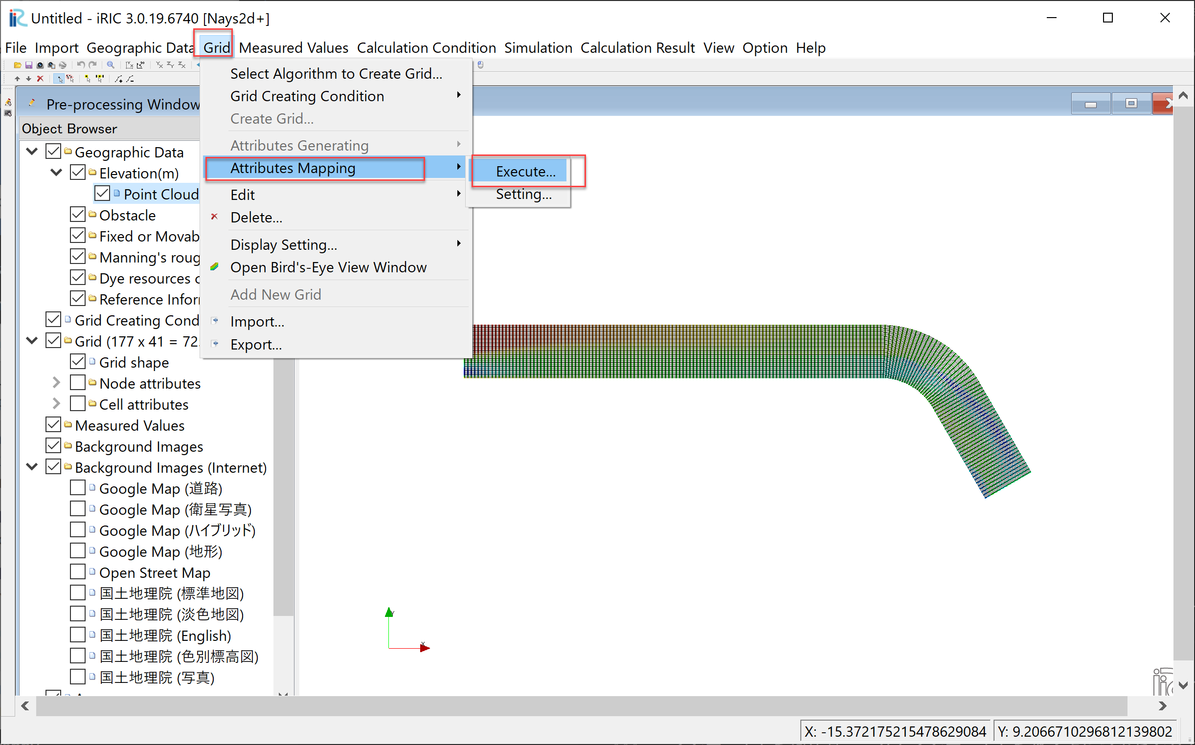
Figure 88 : 「Execute Mapping」

As Figure 89, you will be asked which [Geographic Data] to be mapped. Put check mark in the box of [Elevation(m)], and press [OK].

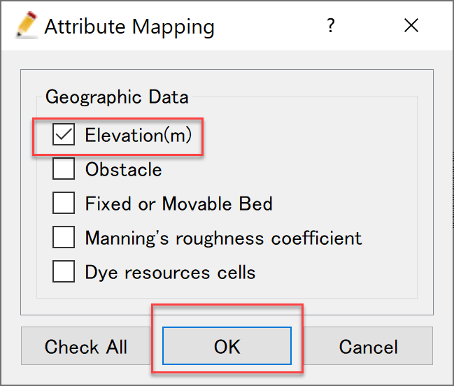
Figure 89 : Selection of the Mapping Item

When the mapping is completed, press [OK] as Figure 90.

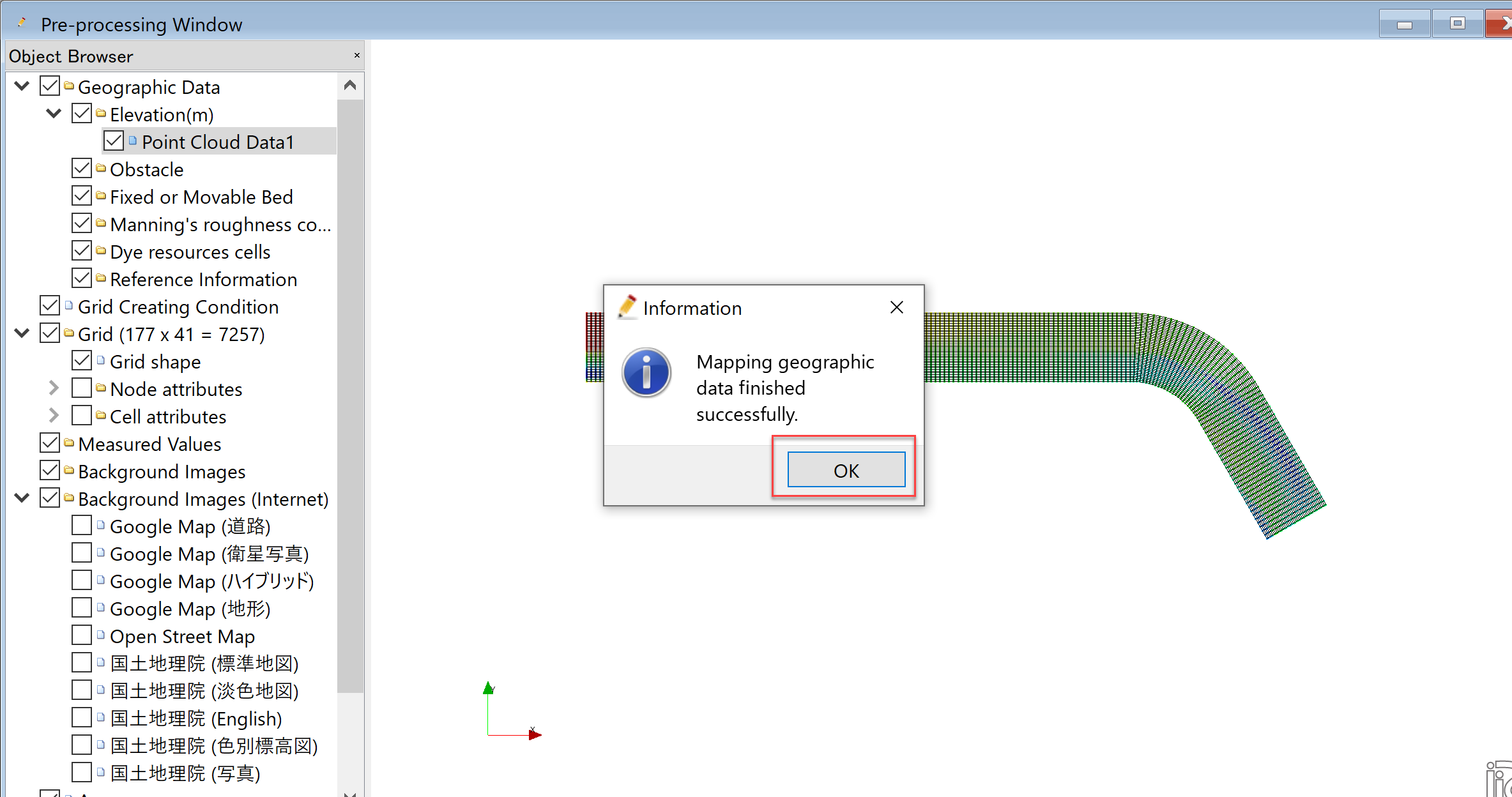
Figure 90 : Mapping Completed

Setting Calculation Condition for Nays2d＋

In the window of [Calculation Condition] which appears when you select [Calculation Condition]->[Setting], set parameters in the [Groups] of [Discharge and downstream water surface elevation], [Time and bed erosion parameters], [Boundary Condition], [Other computational parameters] and [3D Velocity Profile] as, Figure 91, Figure 92, Figure 93, Figure 94, and Figure 95, respectively.

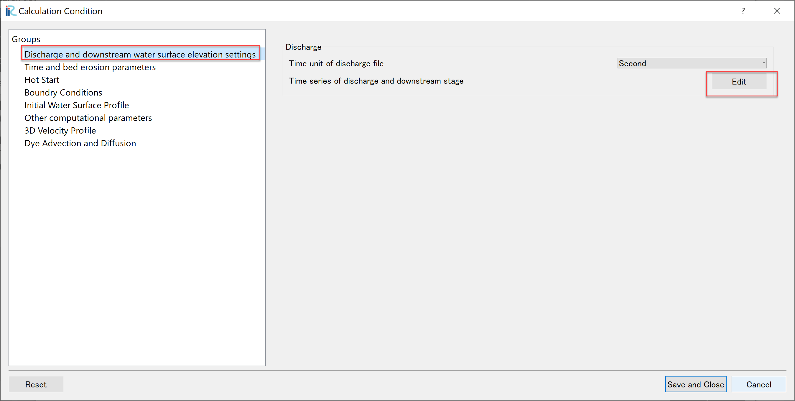
Figure 91 : Discharge and downstream water surface elevation

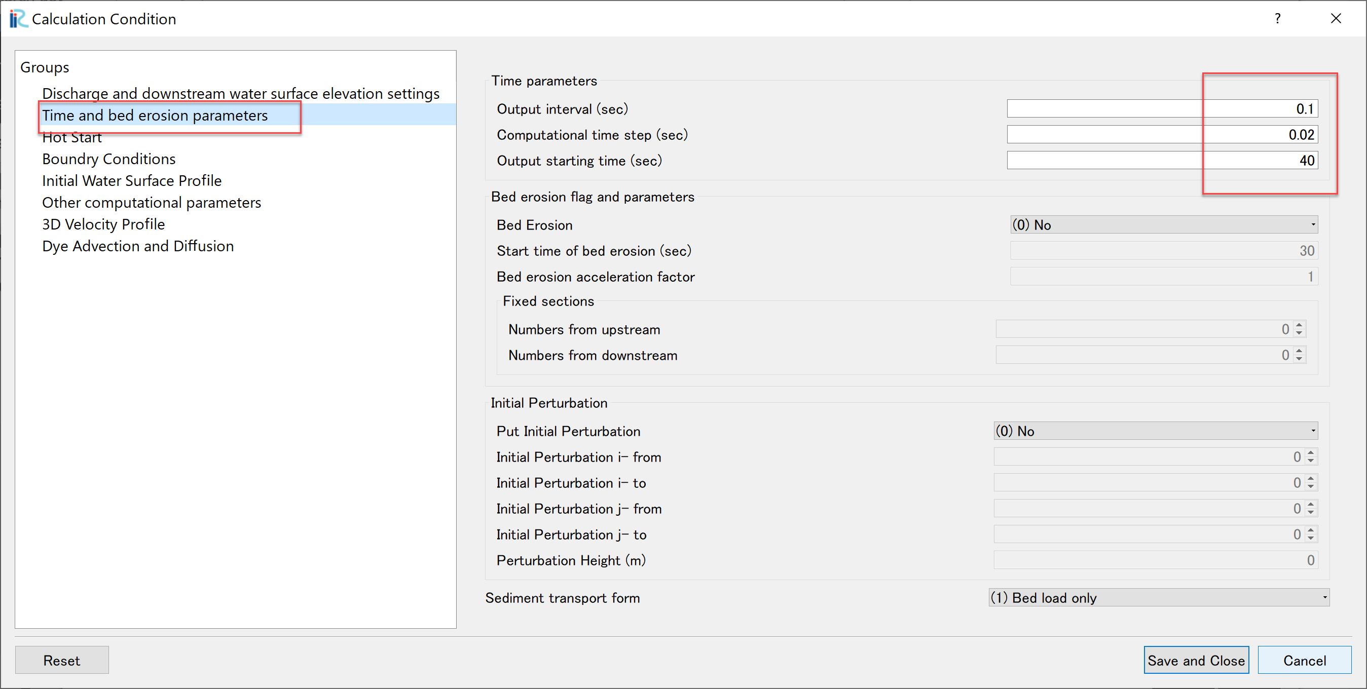
Figure 92 : Time and bed erosion parameters

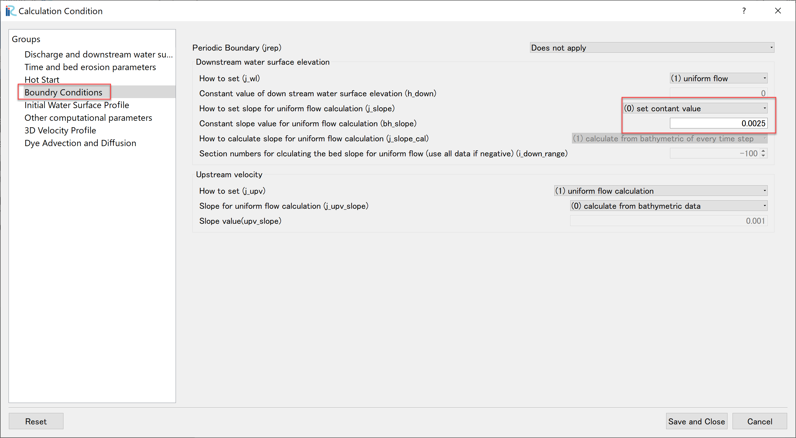
Figure 93 : Boundary Condition

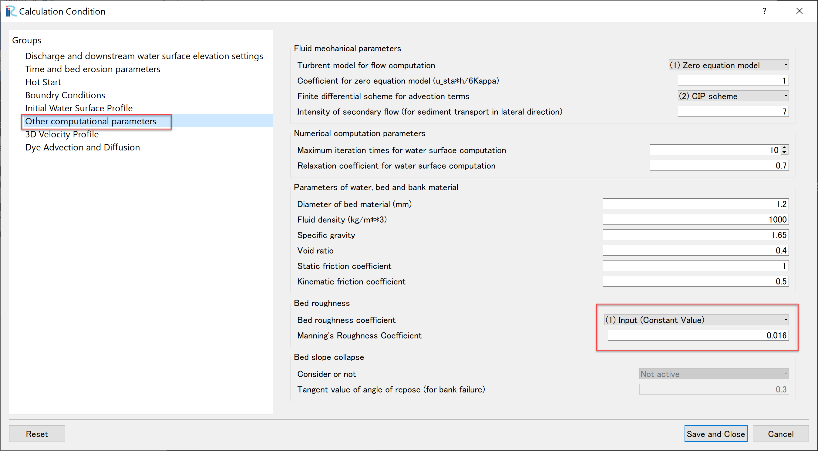
Figure 94 : Other computational parameters

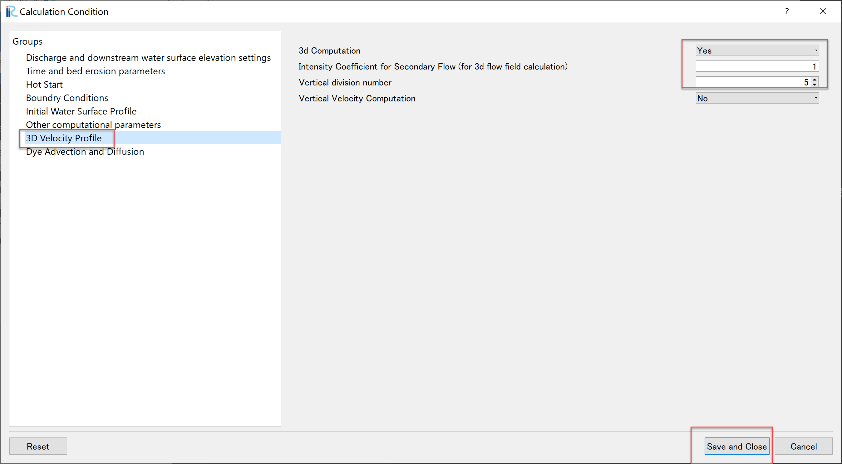
Figure 95 : 3D Velocity Profile

In addition, while in the settings of the [Discharge and downstream water surface elevation], Figure 91, press [Edit] and set discharge data in in the [Time series of discharge and downstream stare] setting window as Figure 96.

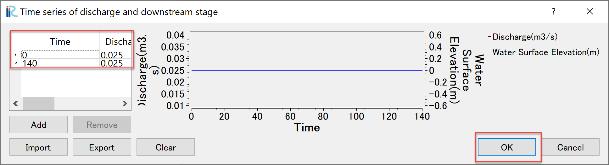
Figure 96 : Setting the time series of discharge Data

When you finish setting all the calculation condition, press [Save and Close] in the [Calculation Condition] window.

Execute Nays2d+

We will skip the explanation of how to executing Nays2d+ because it is exactly same as other solvers. However, it is recommended that you save the project before running the calculation. In this case, we save the file to a project named [Nays2d+Flow].

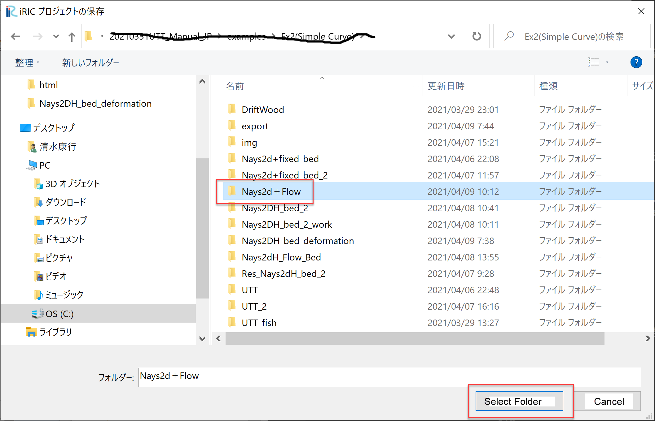
Figure 97 : Save project(Nays2d+Flow)

The results are saved in a CGNS file named [Case1.cgn], which will be used for the tracer tracking computation of UTT as input data. Be sure to save the result using [Calculation Result]->[Save] even when the calculation is finished. (Figure 98).

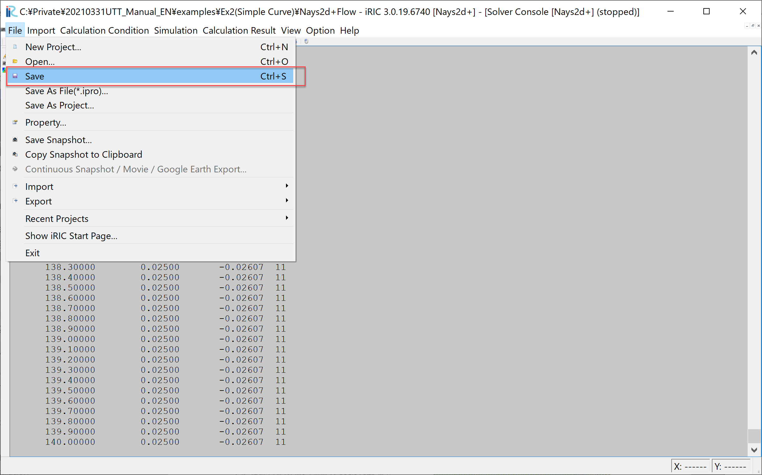
Figure 98 : Save the Results of the Computation (Don’t Forget!)

Tracer Tracking by UTT

Select a Solver

From the iRIC startup screen, select [New Project], and in the solver selection screen appears. Select “UTT” and click “OK” (Figure 99).

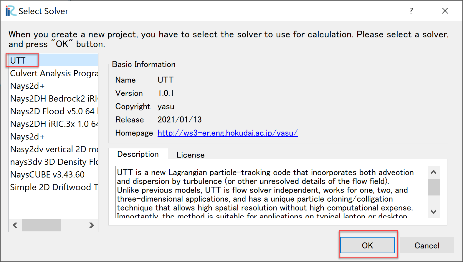
Figure 99 : Select and Launch UTT

Import Grid

Right click [Grid(No Data)] and select [Import] as Figure 100.

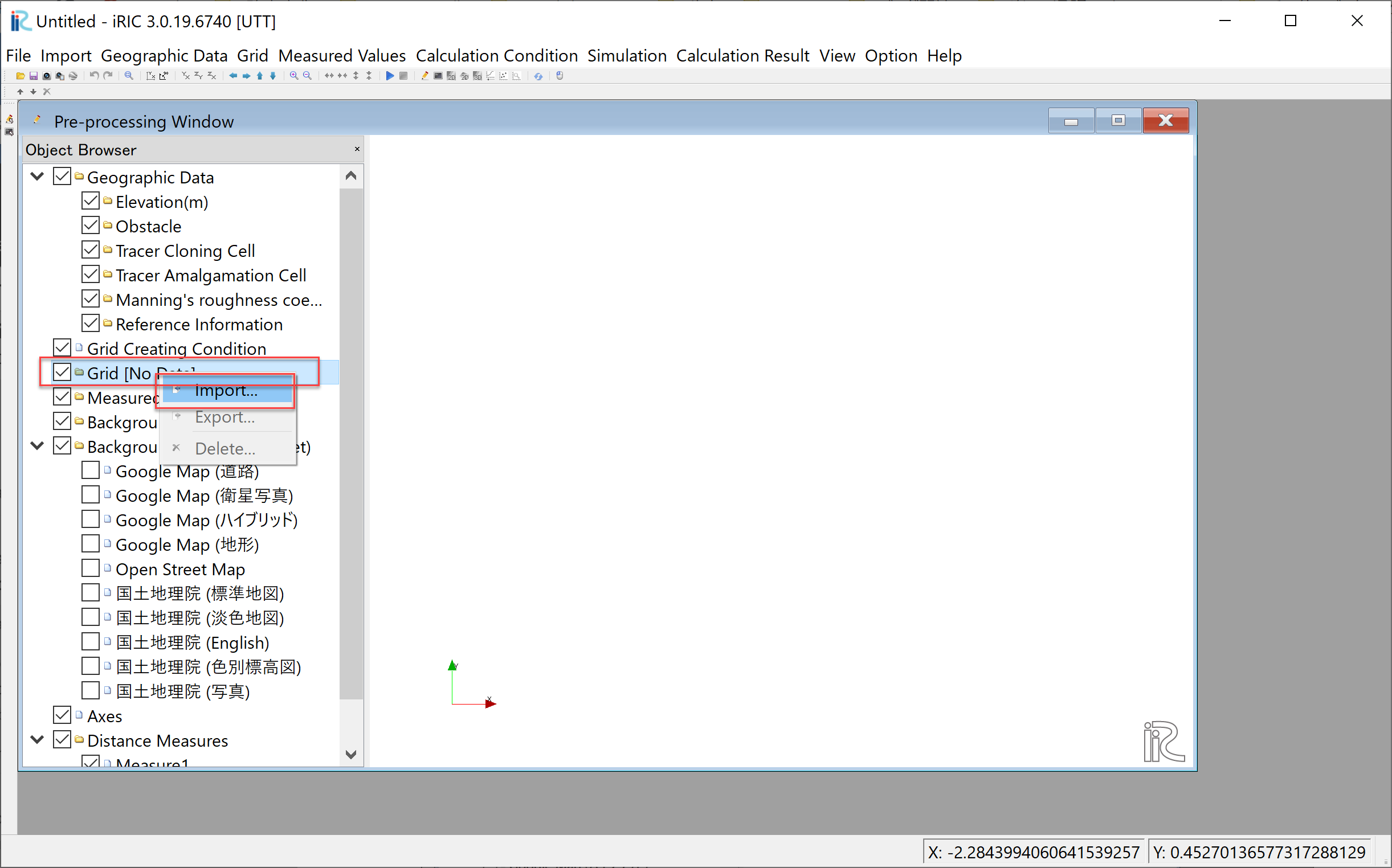
Figure 100 : [Import Grid(1)]

From the [Select Import File] window as Figure 101, choose [Case1.cgn] in the folder [Nays2d+Flow] which is produced by the [Nays2d+] calculation in the previous section.

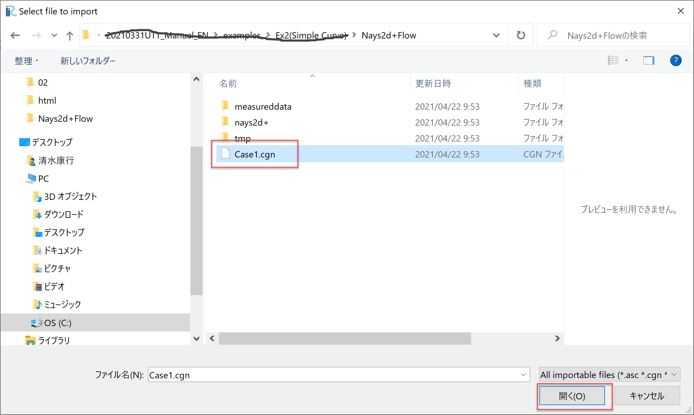
Figure 101 : [Import Grid(2)]

Press [Yes] button when warning message is coming out as Figure 102, and the grid import is completed as Figure 103.

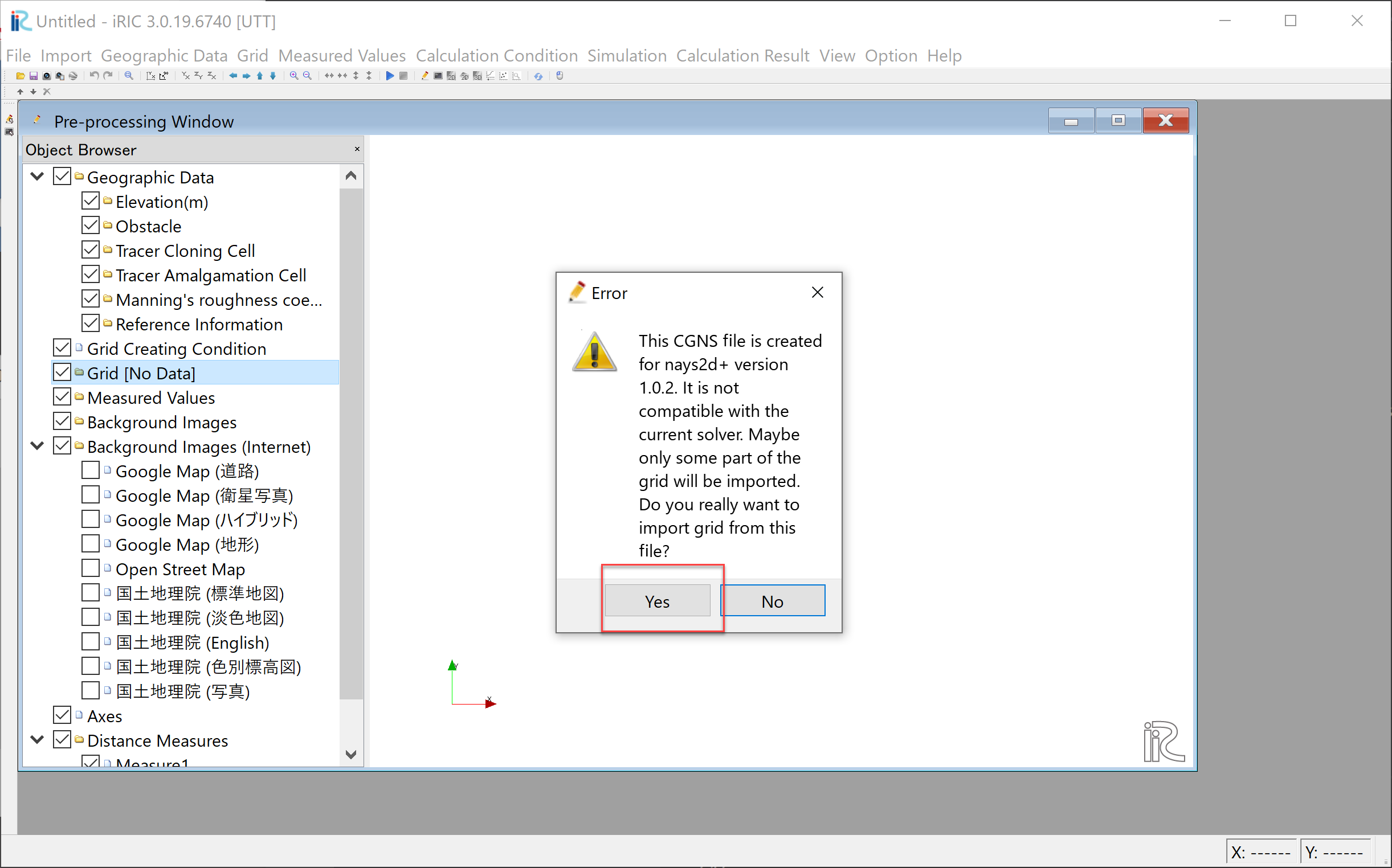
Figure 102 : [Warning Message]

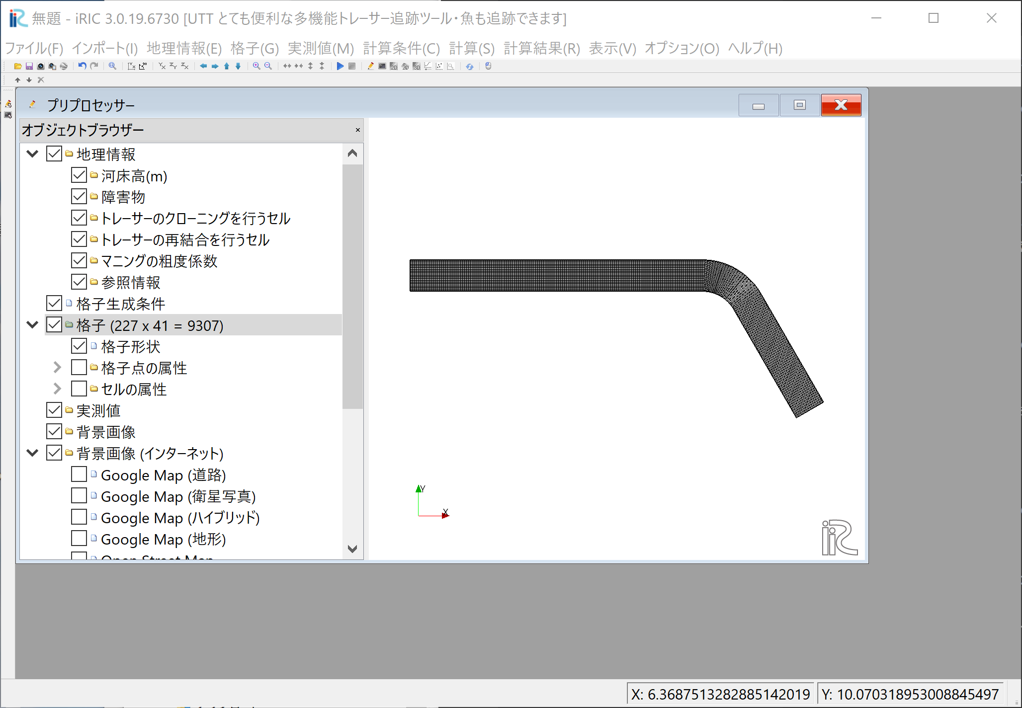
Figure 103 : [Grid Import Completed]

Tracer Tracking Simulation by UTT

Setting Simulation Condition

From the main menu bar, when you select [Calculation condition]->[Setting]. [Calculation Condition] window appears, and in this window, set parameters in the [Groups] of [Basic Settings], [Normal Tracers Supplying Condition] and [Diffusion Condition], as Figure 104, Figure 105, and Figure 106, respectively. In this section, we first perform tracer tracking without considering the effect of sub-grid turbulence.

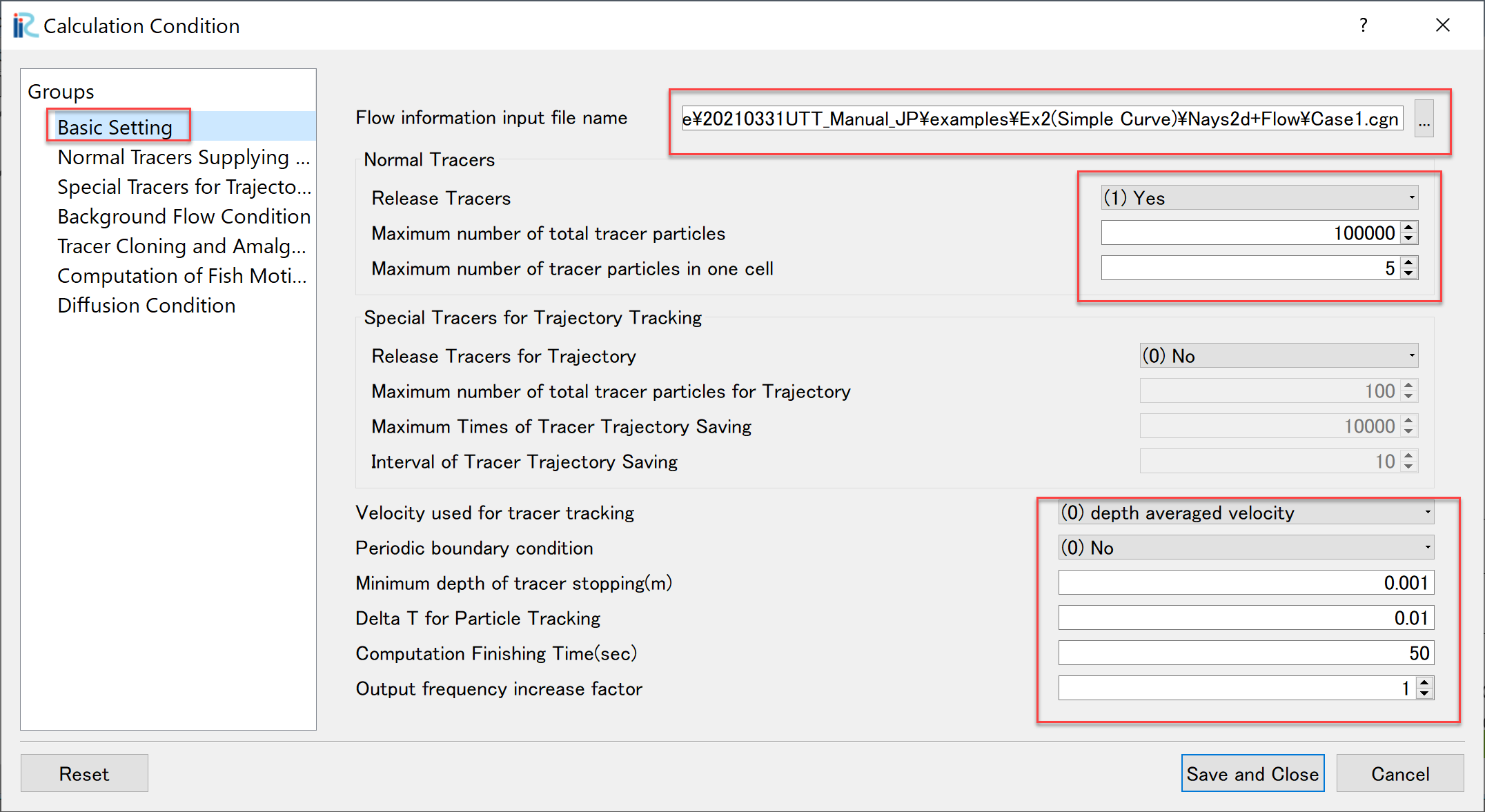
Figure 104 : Basic Settings

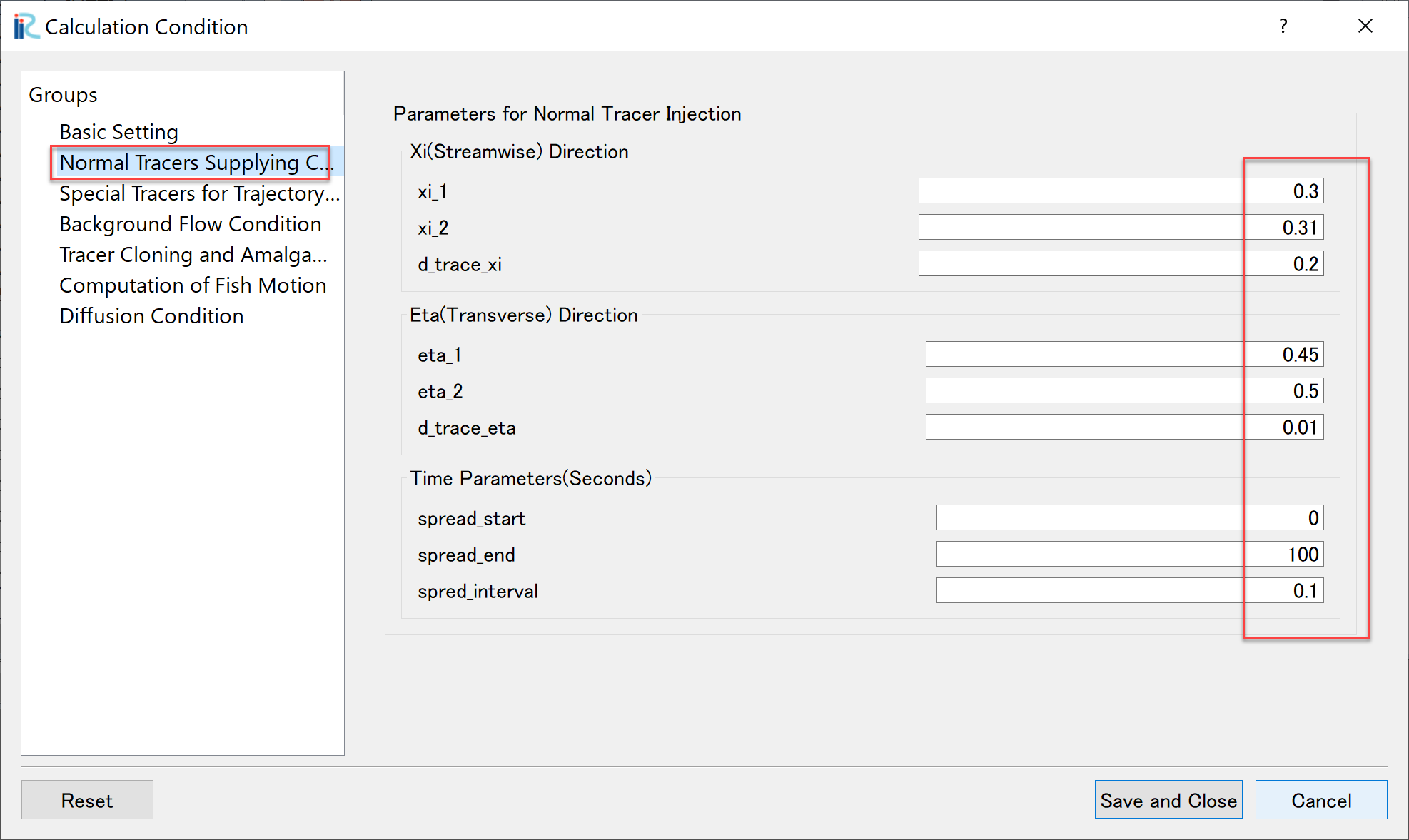
Figure 105 : Normal Tracers Supplying Condition

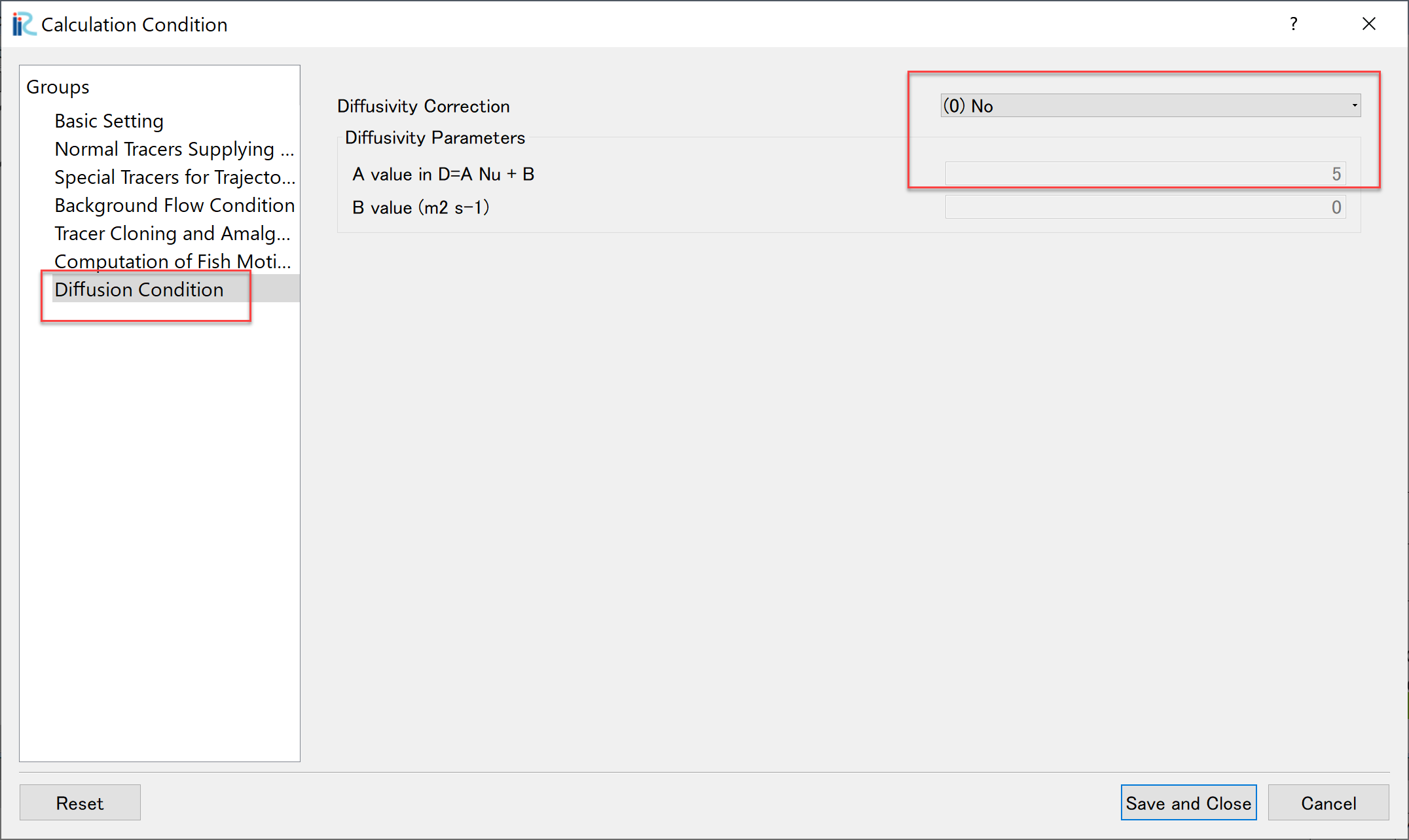
Figure 106 : Diffusion Condition

In addition.Figure 100 The [CGNS file to read the flow calculation results] in the [CGNS file to read the flow calculation results] is the same as the one in the previous section [Flow calculation with Nays2d+]. Select [Case1.cgn] in the [Nays2d+Flow] project folder where you saved the results of ( Figure 103)

In addition, the [Flow information input file] in Figure 104, is the same file with the [Case1.cgn] which was produced by the flow simulation of [Nays2d+] in the previous section (Figure 107).

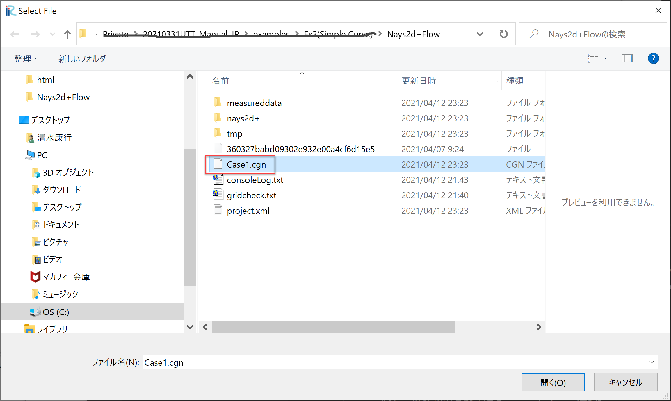
Figure 107 : Assign CGNS file to read flow simulation results

Run UTT

From the main menu, select [Simulation]]->[Run], then you will be asked to save project as usual, save project as recommended. ( Figure 108).

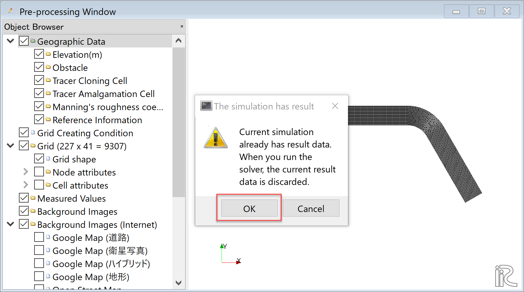
Figure 108 : Saving UTT Project(1)

In the Figure 109, either [Save as file (*.ipro)] or [Save as Project] will do, but in this example, the file is saved as [UTT1.ipro].

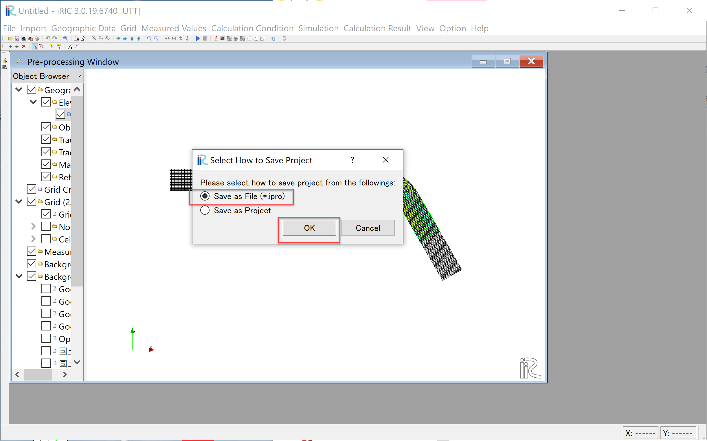
Figure 109 : Saving UTT Project(2)

When the computation starts, Figure 110 appears, and when the computation finishes, Figure 111 appears. Press [OK] to finish computation.

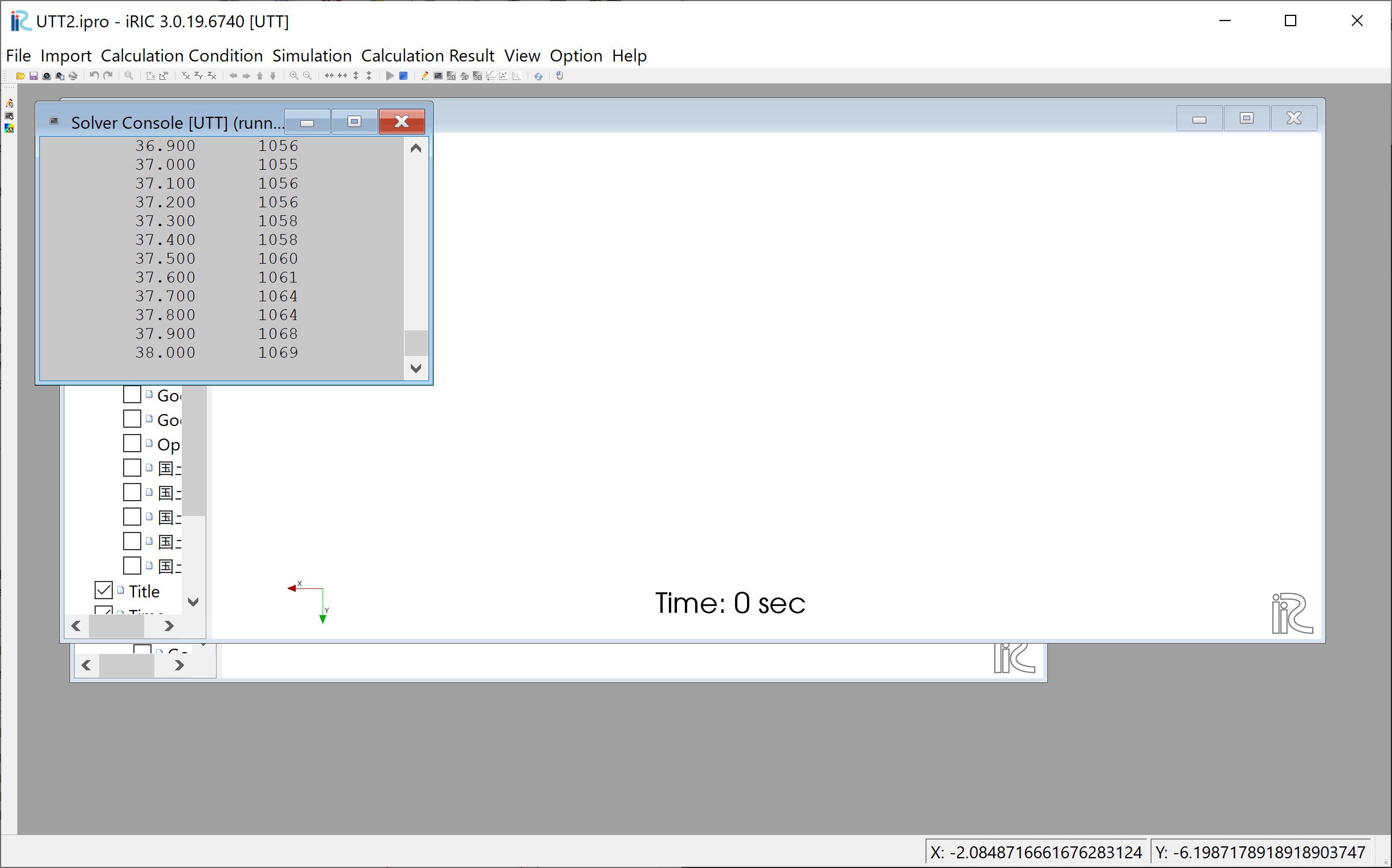
Figure 110 : Execution of UTT(1)

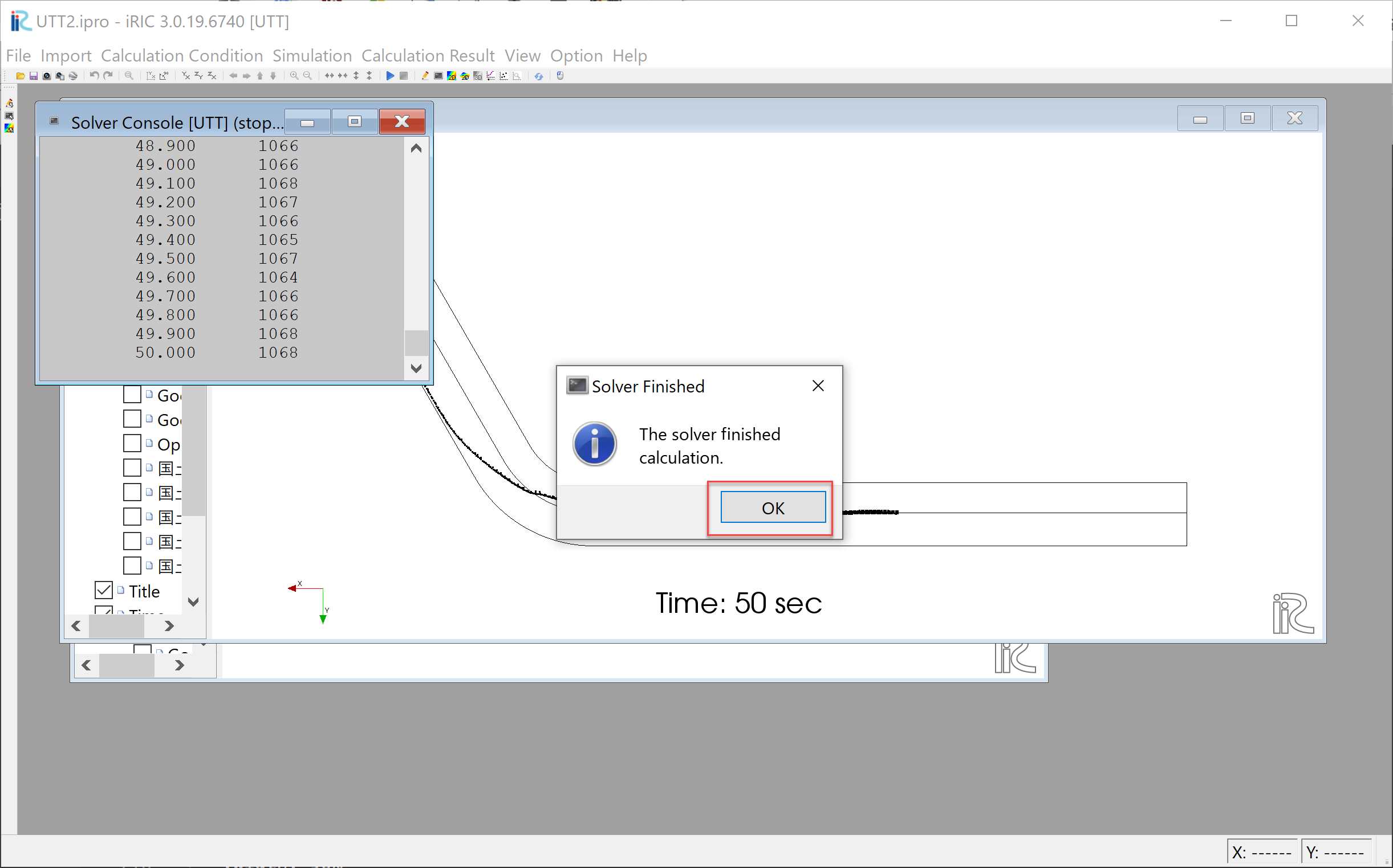
Figure 111 : Execution of UTT(2)

Showing the Results of UTT

From the main menu, select [Calculation Result]->[Open new 2D Post Processing Window], and the calculation results are shown (Figure 112)

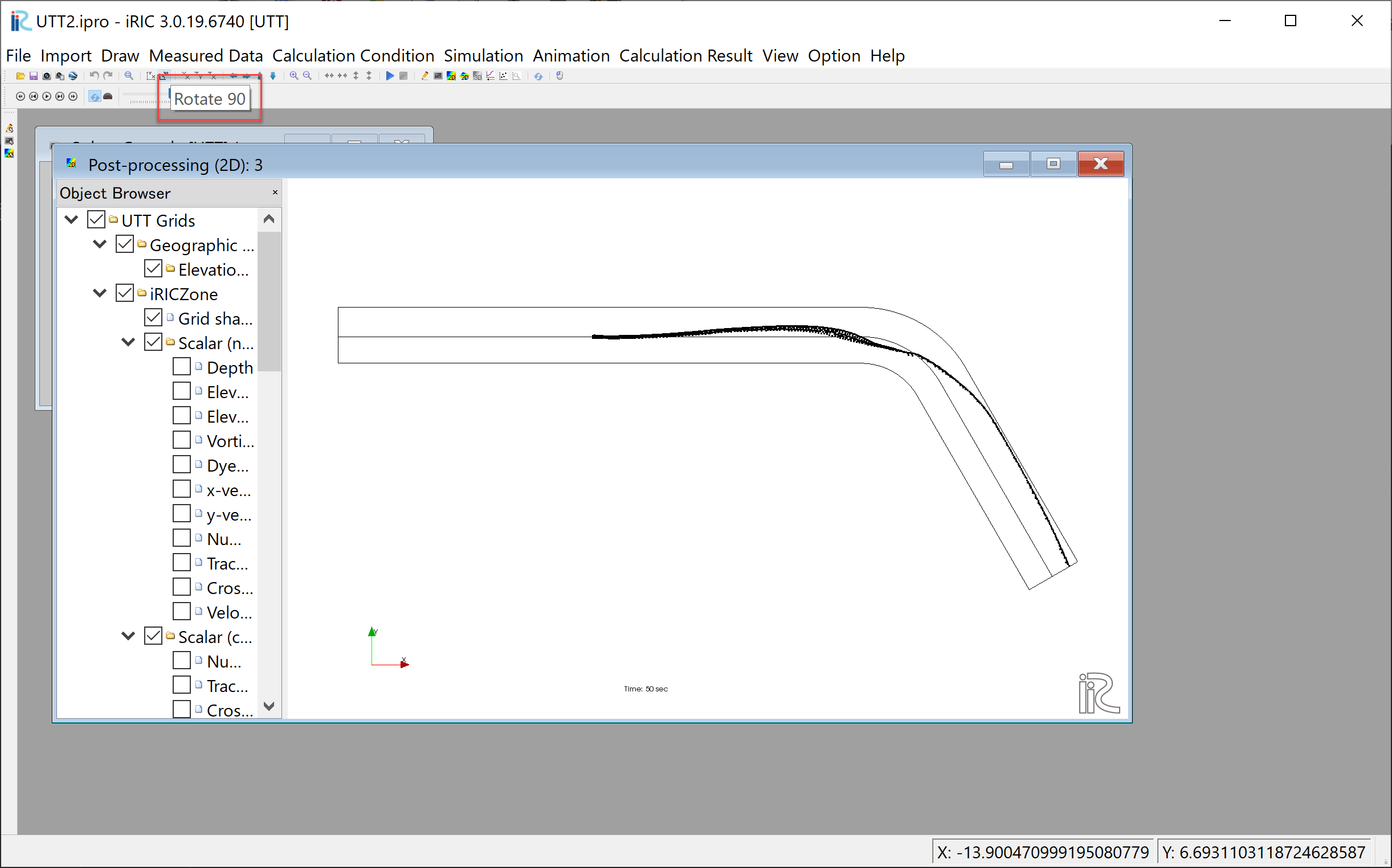
Figure 112 : [2D Post Processing Window]

Since the orientation of the Figure 112 is the opposite to the experimental image shown at the beginning of this chapter Figure 51, press the 90° rotation mark twice to rotate 180° (Figure 113).

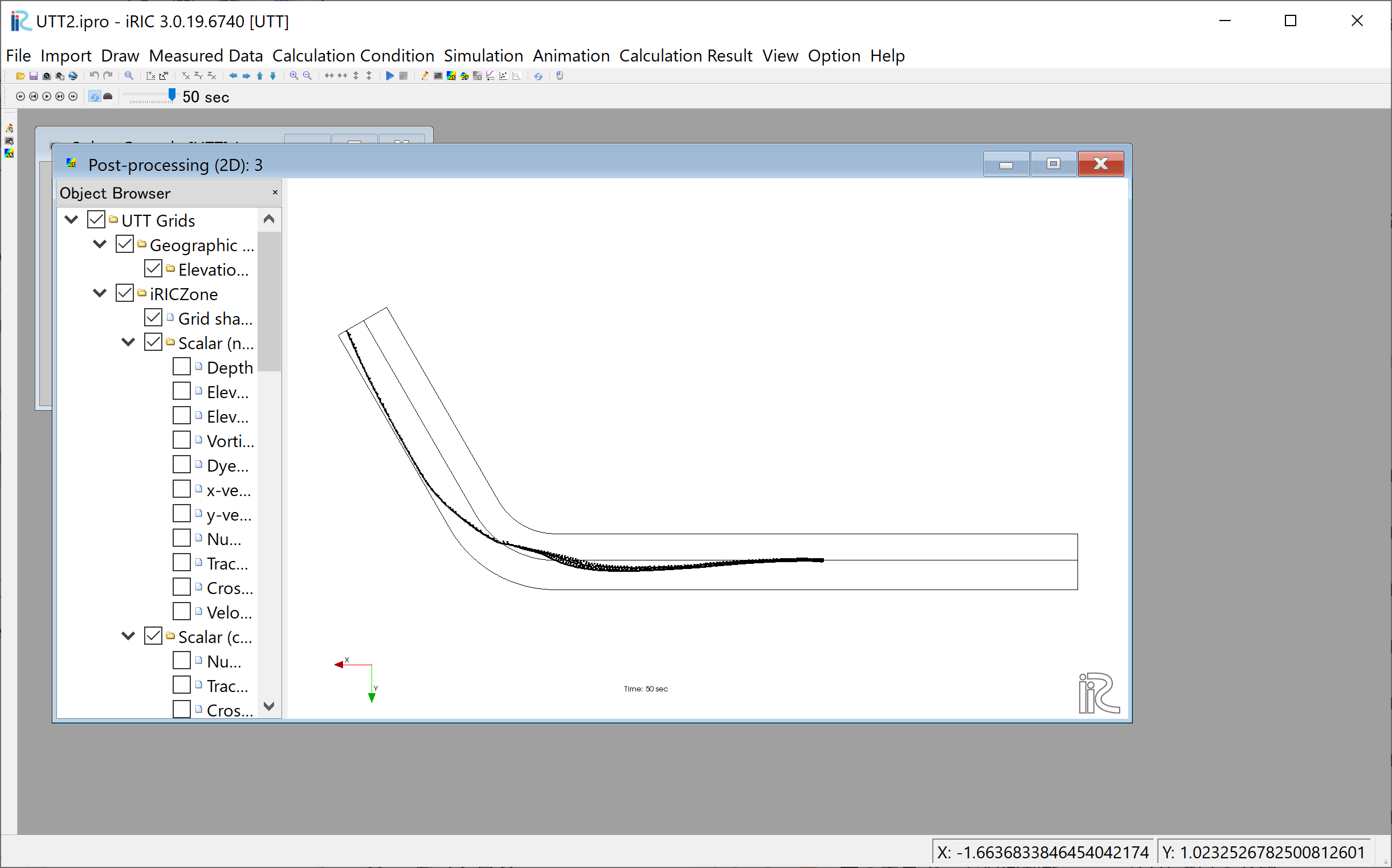
Figure 113 : 2D Post Processing Window 180° rotate

Since the [Time] display is so small that it’s hard to see, select [Time]->[Properties] in the object browser (Figure 114), display [Time Setting] and set the font size appropriately large (Figure 115).

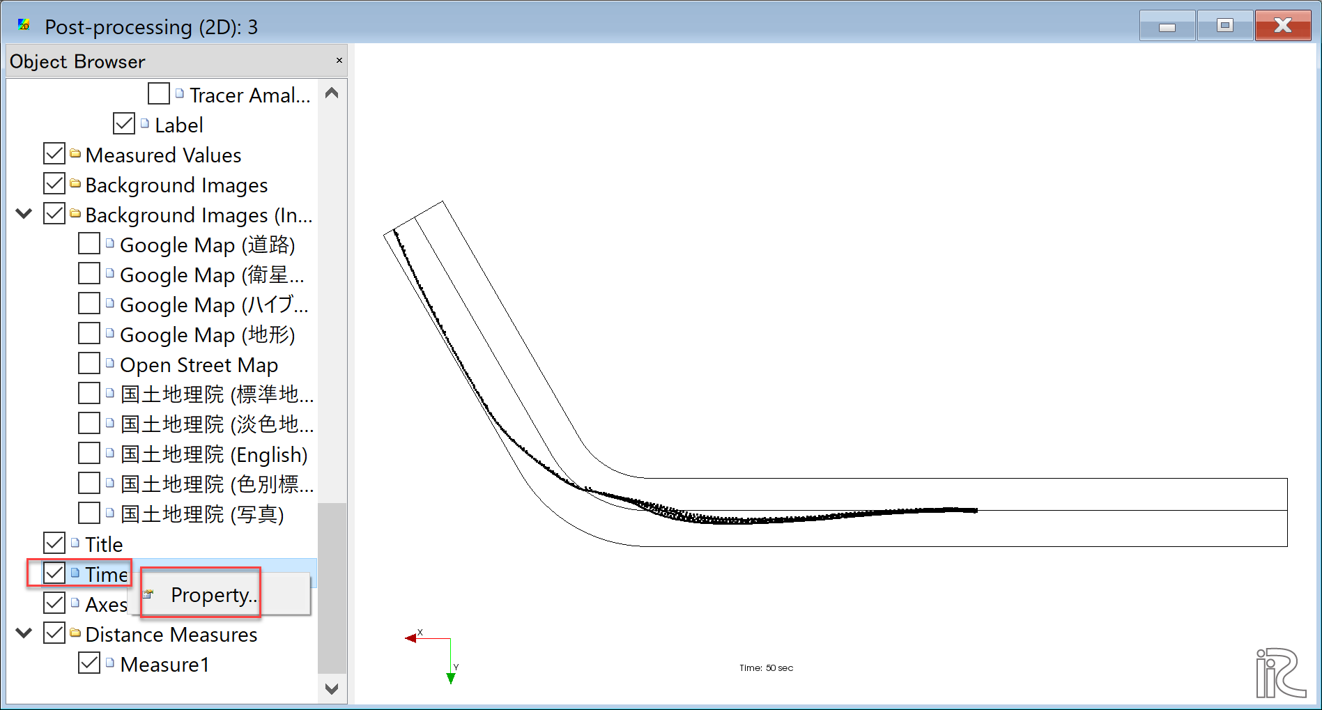
Figure 114 : Time Setting(1)

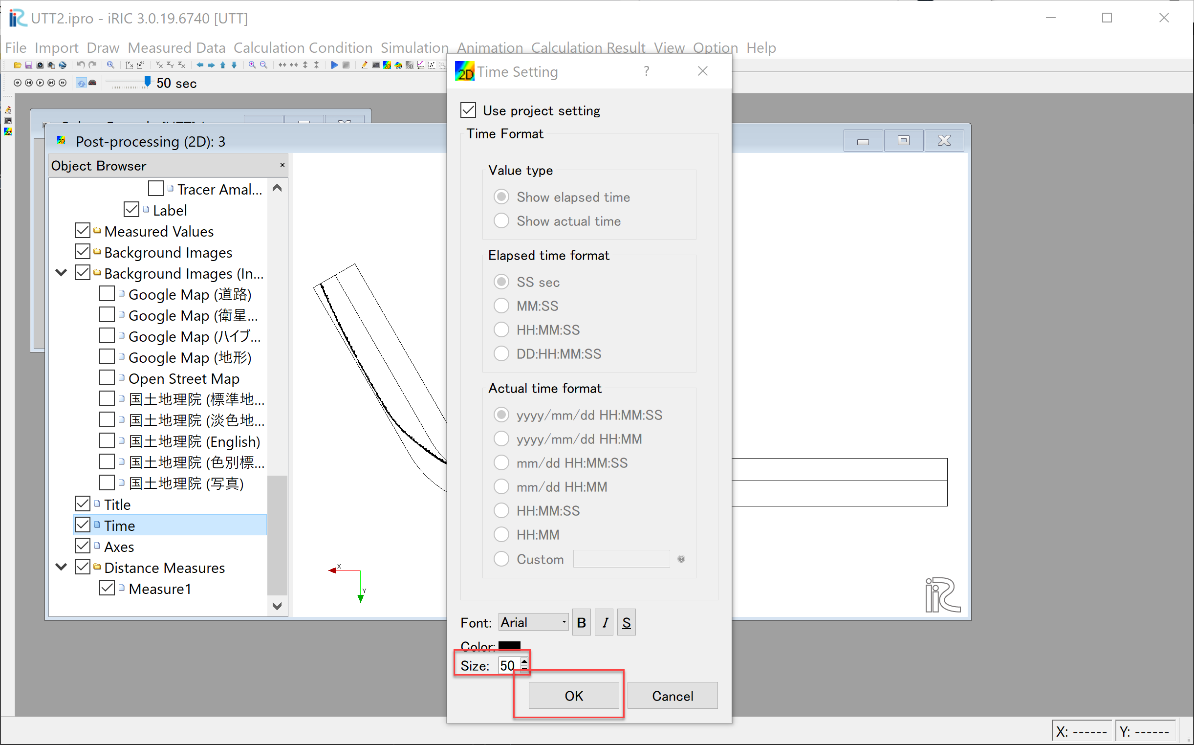
Figure 115 : Time Setting(2)

As shown in Figure 116, put time bar back to 0, and from the main menu, select [Animation]->[Start/Stop], then the animation starts( Figure 117).

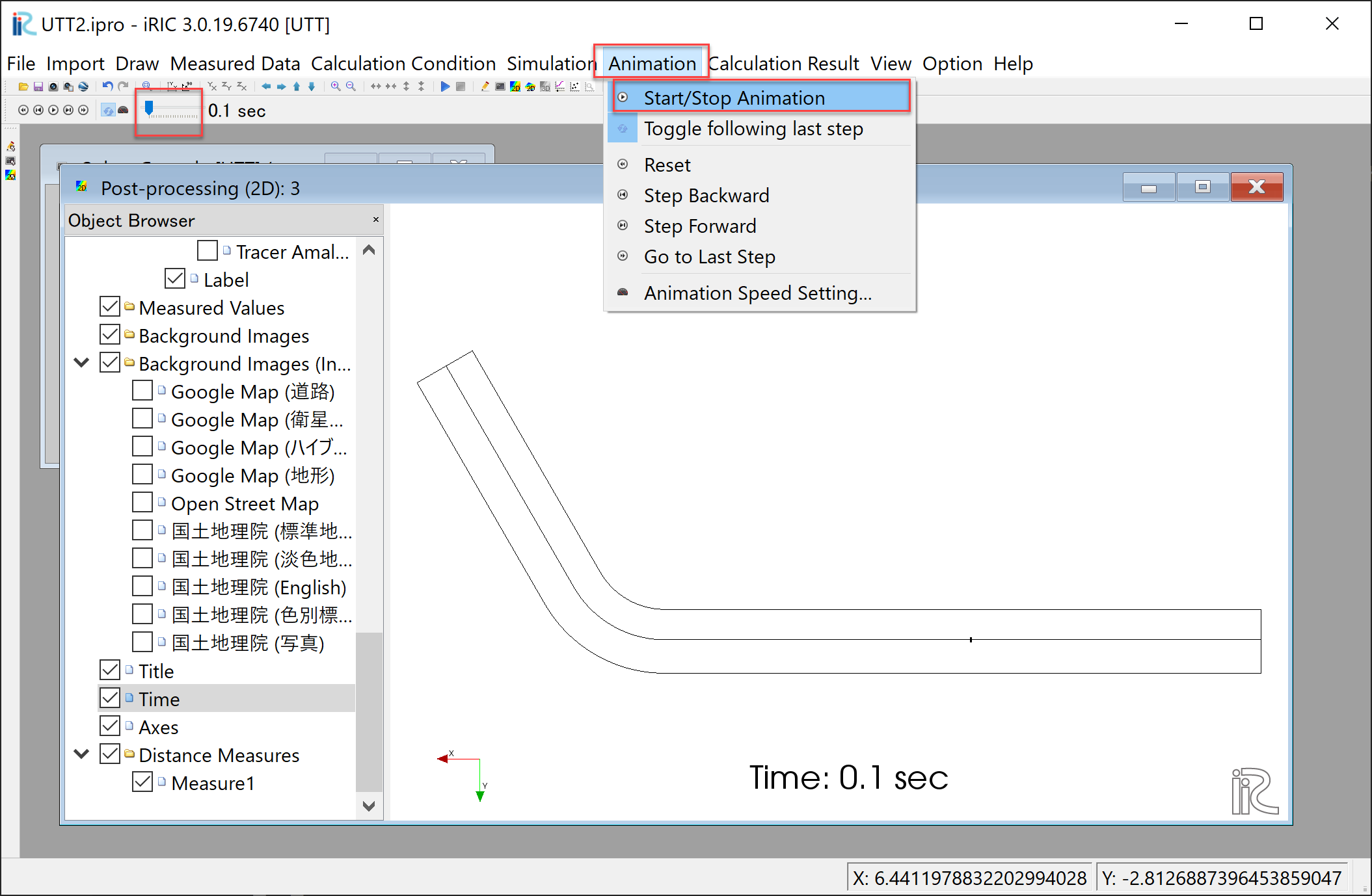
Figure 116 : Starting Animation

Figure 117 : Tracer Animation (Turbulent Diffusivity A=0)

There is almost no diffusion and the tracers are just flowing straightly.

Comparison of the Turbulent Diffusivity

Select [Calculation Condition]->[Setting] and open [Calculation Condition] window. As shown in Figure 118, set in the [Group]->[Diffusion Condition], [Diffusivity Correction]->[Yes] and set the value [A=1] of the [Diffusivity Parameter]

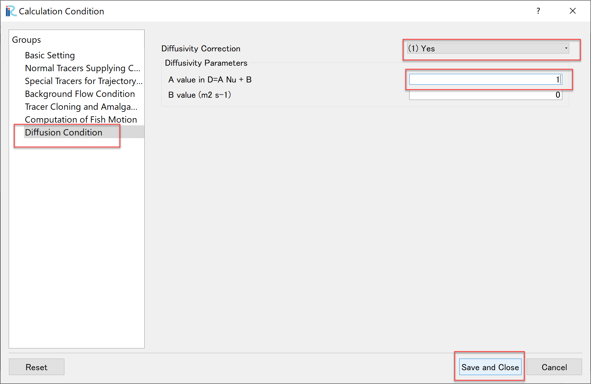
Figure 118 : Random Walk Parameter Setting (A=1)

Figure 119 : Animation of the Tracer Motion (A=1)

In the same manner，if we do the simulation with [A=5], [A=10] and [A=50], the results becomes as Figure 120, Figure 121 and Figure 122.

Figure 120 : Animation of the Tracer Motion (A=5)

Figure 121 : Animation of the Tracer Motion (A=10)

Figure 122 : Animation of the Tracer Motion (A=50)

When we compared with the experimental results of the Figure 51, it seem that the case with A=10, Figure 121, is the closest to the experiment.

Cloning of the Tracers

In the main menu, select [Calculation Condition]->[Setting] to show [Calculation Condition]. In the [Calculation Condition] window, select [Tracer Cloning and Amalgamation], set parameters as Figure 123. Select [Diffusion Condition] and set [A=1] and press[Save and Close] as Figure 124. Then execute the UTT solver by choosing [Simulation]->[Run], and show the results (Figure 125).

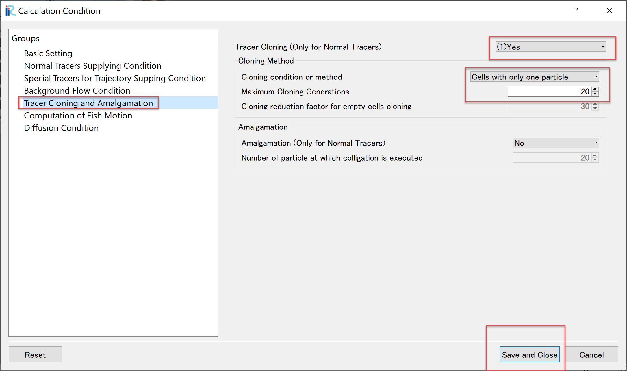
Figure 123 : Setting the Tracer Cloning(1)

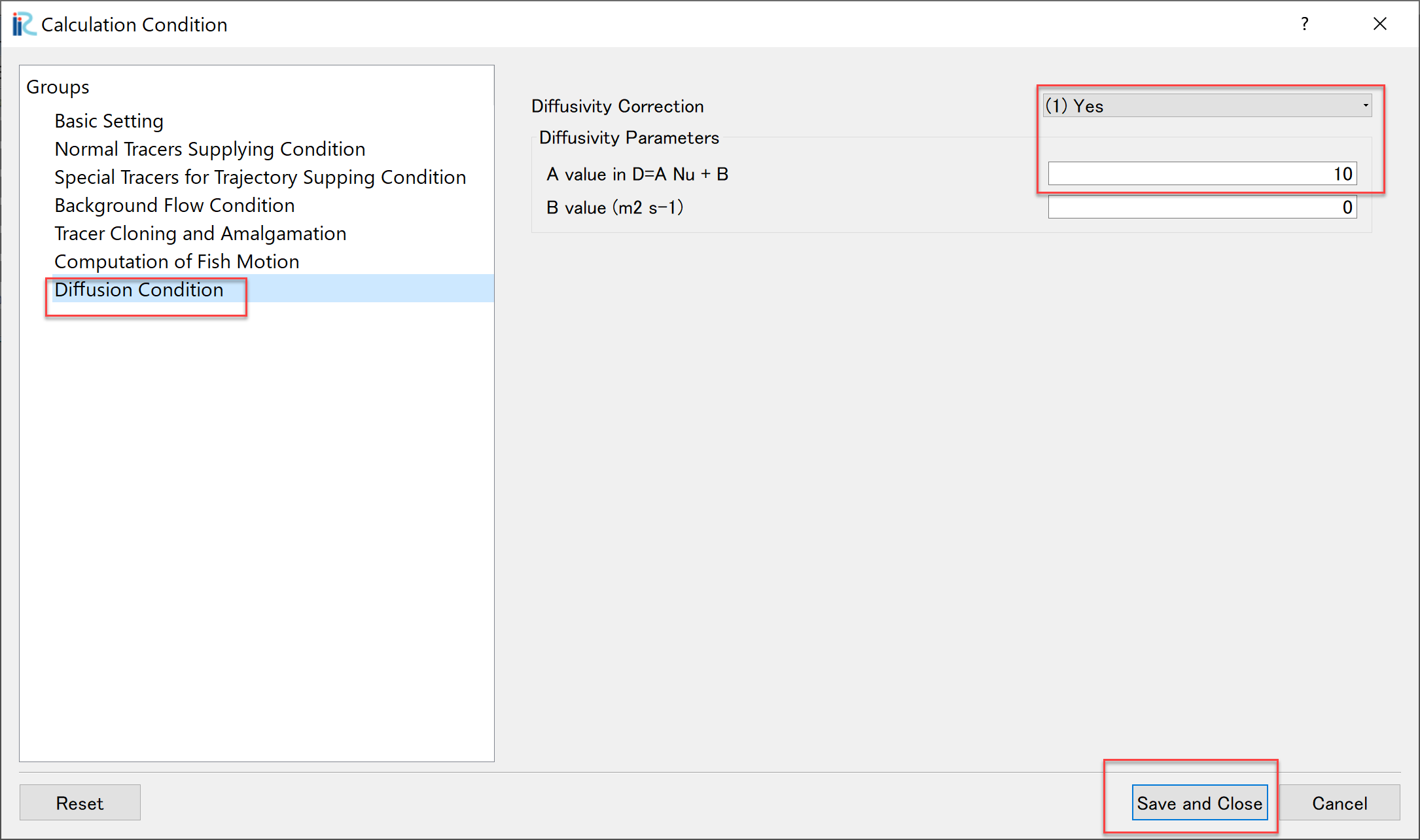
Figure 124 : Setting the Tracer Cloning(2)

Figure 125 : Animation of Tracer Cloning (Maximum Generation 20，A=10)

The spread range of the tracers in Figure 51 is close to the diffusion range of the green dye in the experimental movie. The number of tracers appears to be enormous, but if you put check marks in [Particles]->[Scalars]->[Generations] in the object browser, generations of the tracers are displayed as Figure 126.

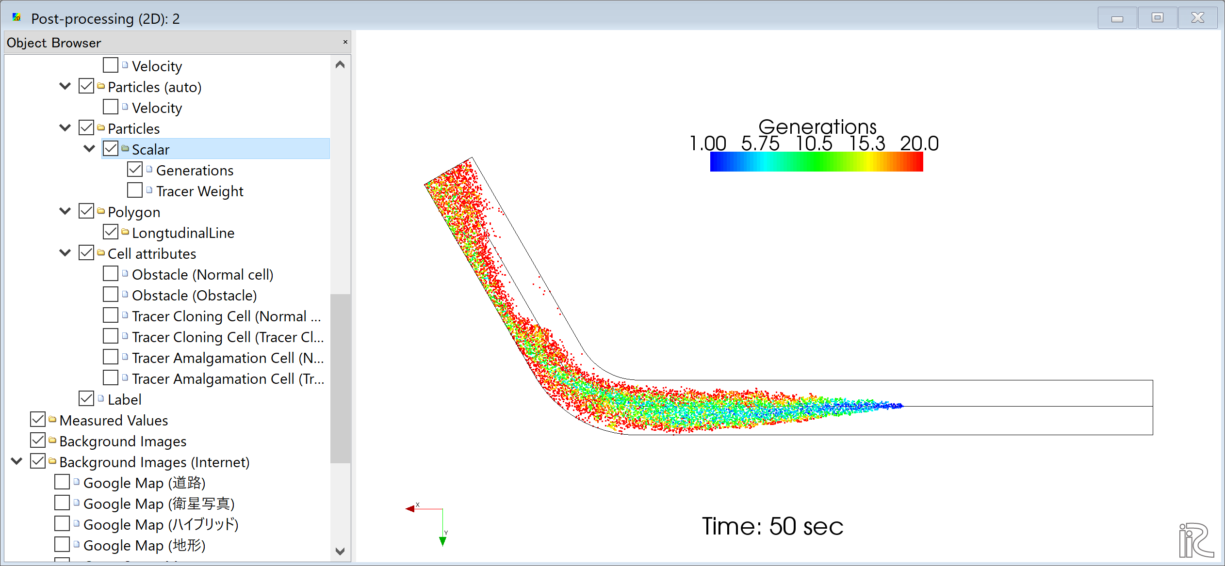
Figure 126 : Color-coded View of the Clone Generations

When this is animated, it becomes as Figure 127.

Figure 127 : Tracers Clone Animation(Maximum 20 Generations，A=10, Color-coded View)

As described in Overview , the substantial weight in the 10th generation is W=0.00195, and in the 20th generation is W=0.00000195. Therefore, Figure 126, the concentrations of the tracers of green, yellow, red, etc. are logarithmically lower than that of the central blue tracers. To see the real concentration, the substantial concentration in each cell is visualized by the following procedure.

1. Uncheck the check box at [Scalar] in the object browser (Figure 128).

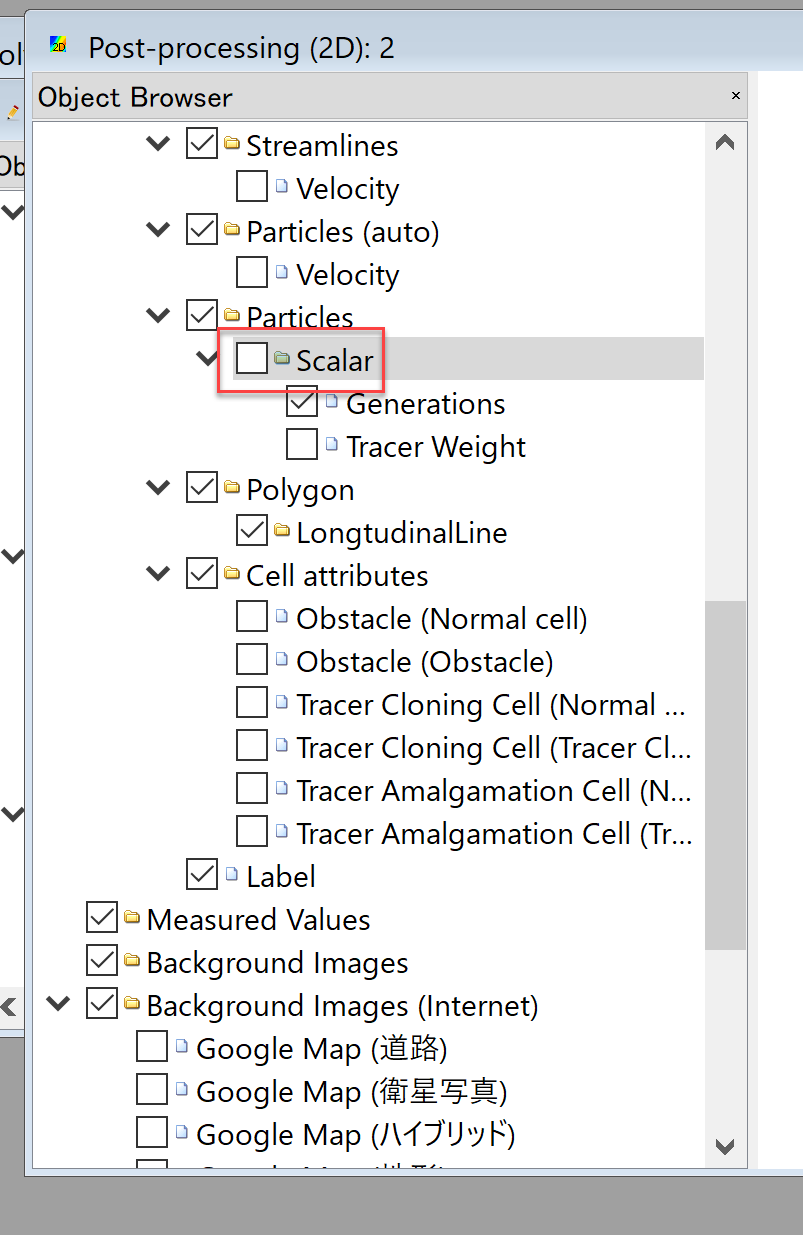
Figure 128 : Uncheck the check box by [Scalar]

2. Put check mark at [Scalar(Cell Center)] and [Weighted numbers of tracers] in the Object Browser (Figure 129).

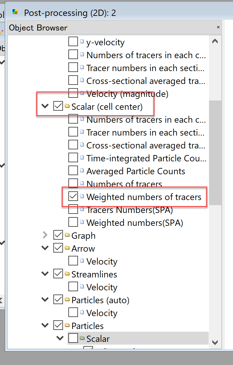
Figure 129 : Put check mark at [Weighted numbers of tracers]

3. Right click [Weighted numbers of tracers] and press [Property]

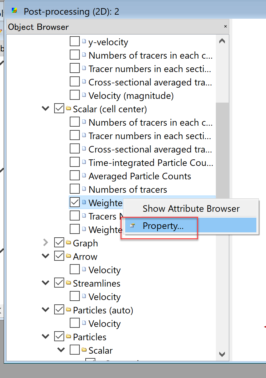
Figure 130 : [Weighted numbers of tracers]->[Property]

4. In the [Scalar Setting] window，uncheck mart at [Auto]，set [Max=0.1] and [Min61e-08]，remove the check mark at [Fill Lower Area]， set [Color map] as [Manual], and press [Setting]．

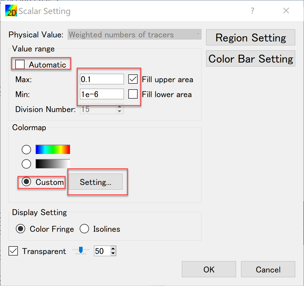
Figure 131 : Scalar Settings

5. In the [Custom Color Map] window，set [Type] [3 Colors], [Maximum Value] as [Dark Green], [Medium Value] as [Light Green] and [1e-06], [Minimum Value] as [White] and press [OK]．

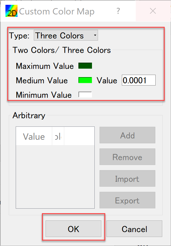
Figure 132 : Custom Color Settings

6. When the window got back to the [Scalar Settings], press [OK] to finish．

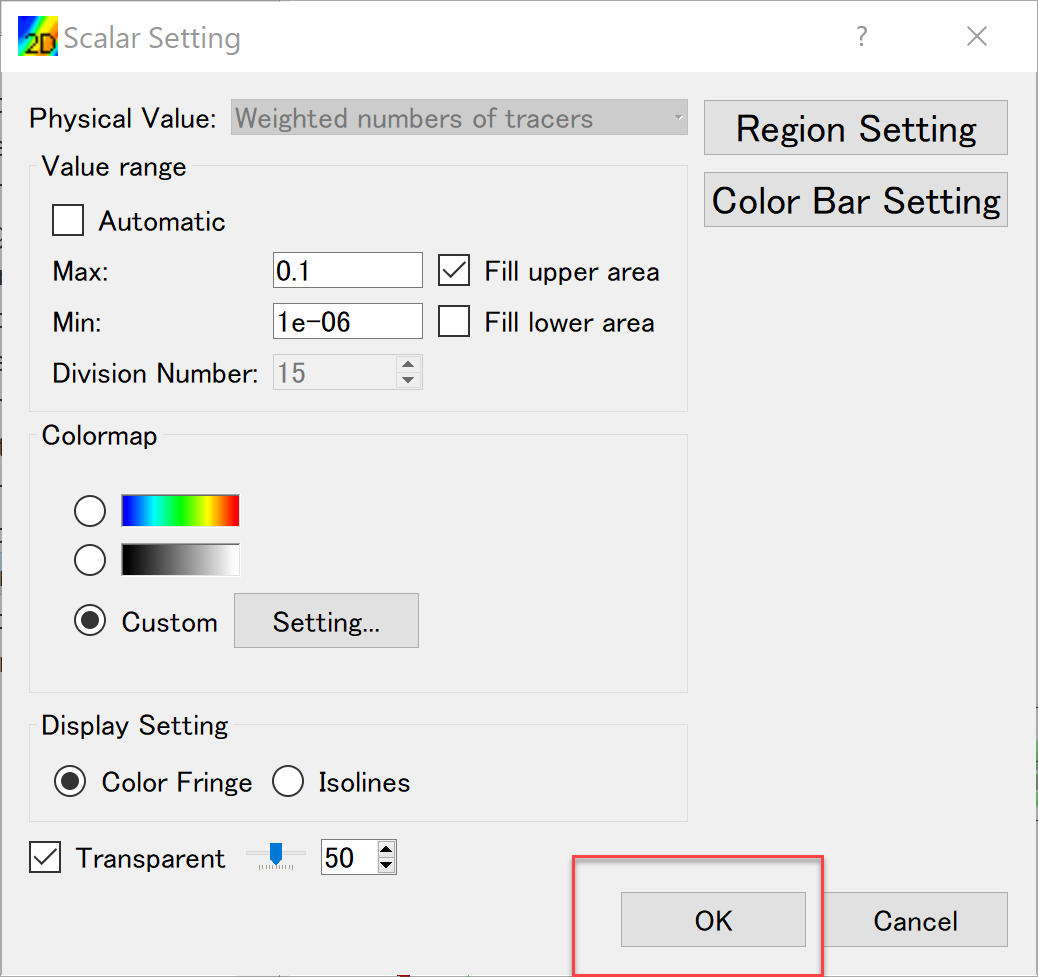
Figure 133 : Scalar Setting (finished)

In the [Post processing (2D)] window, Figure 134, put time bar back to zero, select [Animation]->[Start/Stop], and start animation as Figure 135.

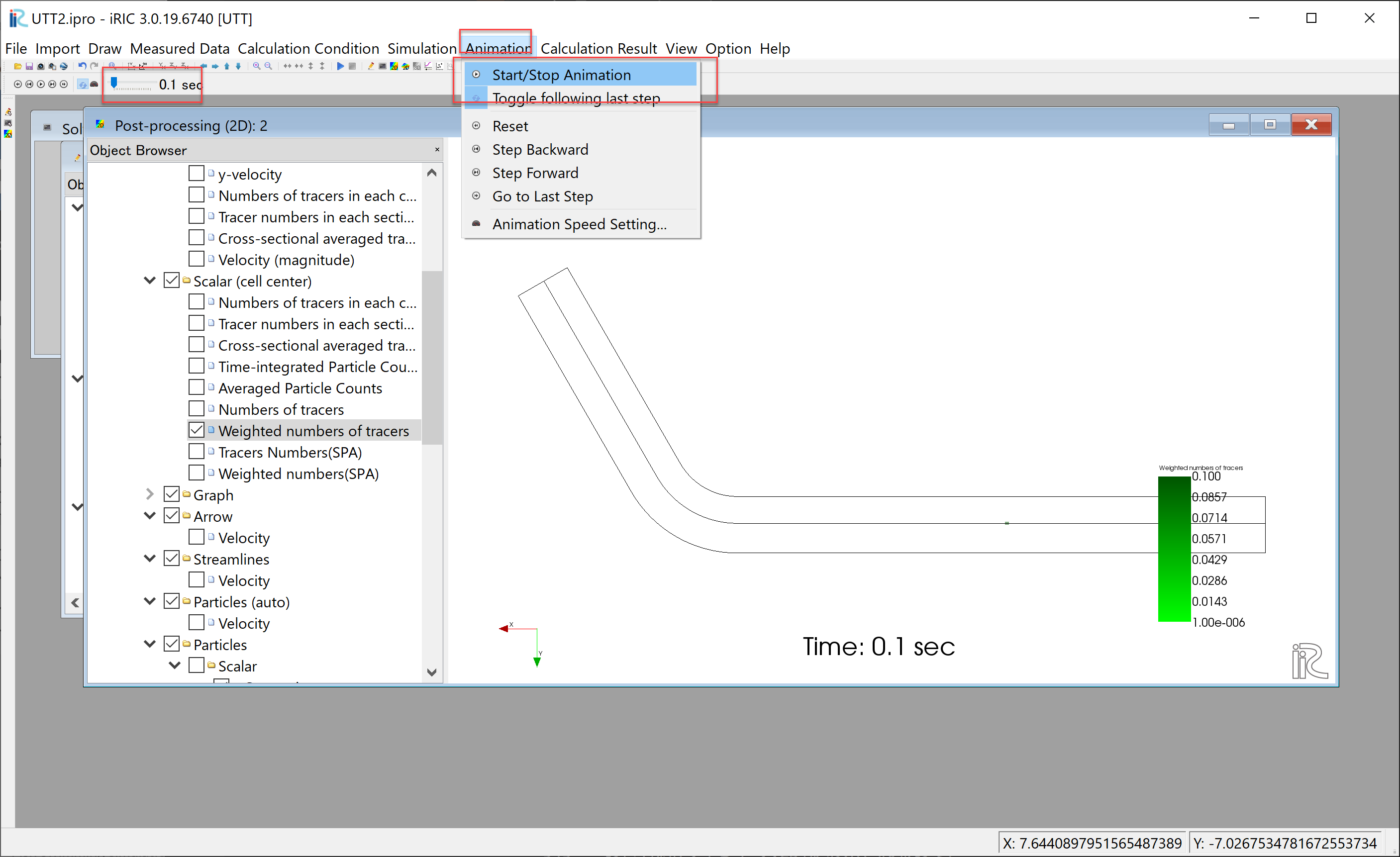
Figure 134 : Starting Animation

Figure 135 : Animation of the tracer concentration considering the weight

The diffusion situation is similar to that of the green dye in the experimental movie of Figure 51.

Flow Visualization using Tracer Cloning

Flow visualization using tracer cloning is shown in this section. In the main menu, click [Calculation Condition], and set parameters in the [Group] of [Normal Tracers Supplying Condition] and [Tracer Cloning and Amalgamation] as Figure 136 and Figure 137, respectively, and press [Save and CLose].

Figure 136

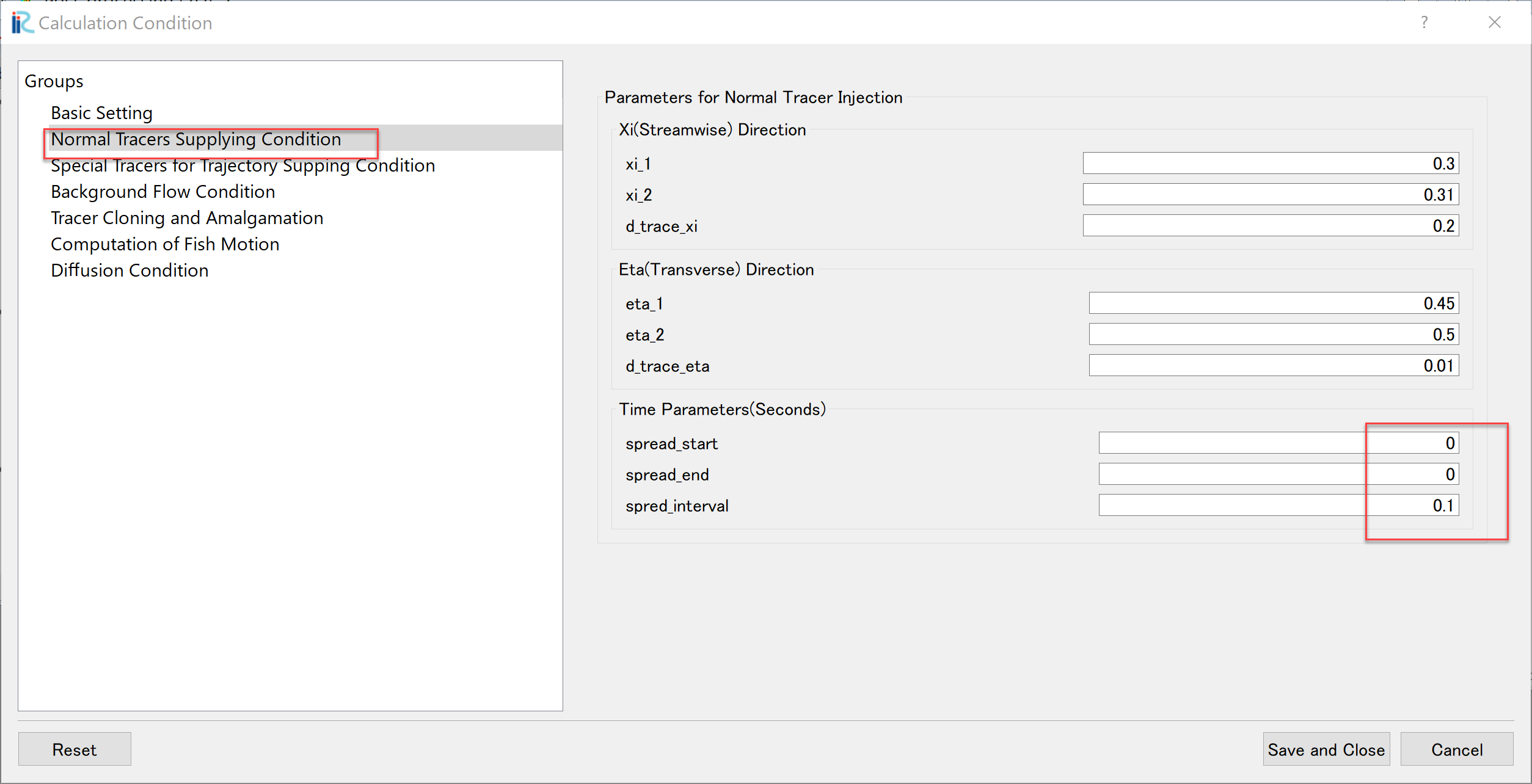
Figure 136 : Calculation Condition Setting(1)

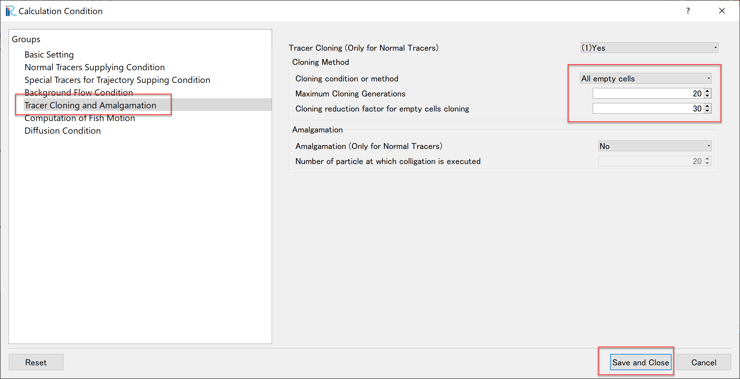
Figure 137 : Calculation Condition Setting(2)

Then after running the UTT solver. in the [Object Browser], remove check mark from [Weighted numbers of tracers], put check marks in boxes at [Particles], [Scalar] and remove the check mark form the [Generation].

From the main menu, select [Animation]->[Srat/Stop], and the animation with evenly distributed tracers in the whole channel is visualized.

Figure 138 : Flow Visualization with Virtual tracers

Swimming Fish Simulation

Set the following parameters in the [Computation of Fish Motion] in the [Calculation Condition] window menu followed by selecting [Calculation Condition]->[Setting] in the main menu.

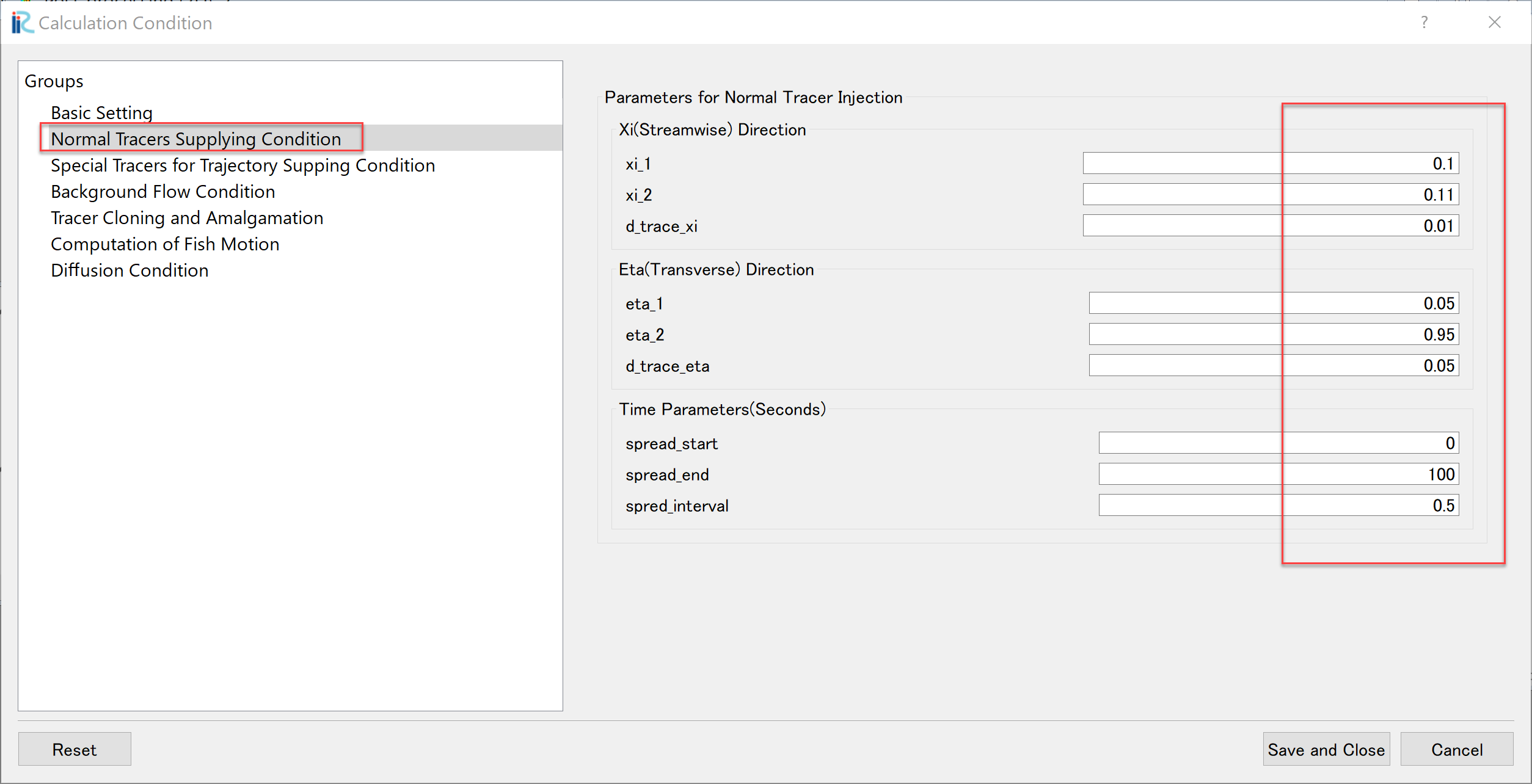
Figure 139 : Setting Condition or Fish(1)

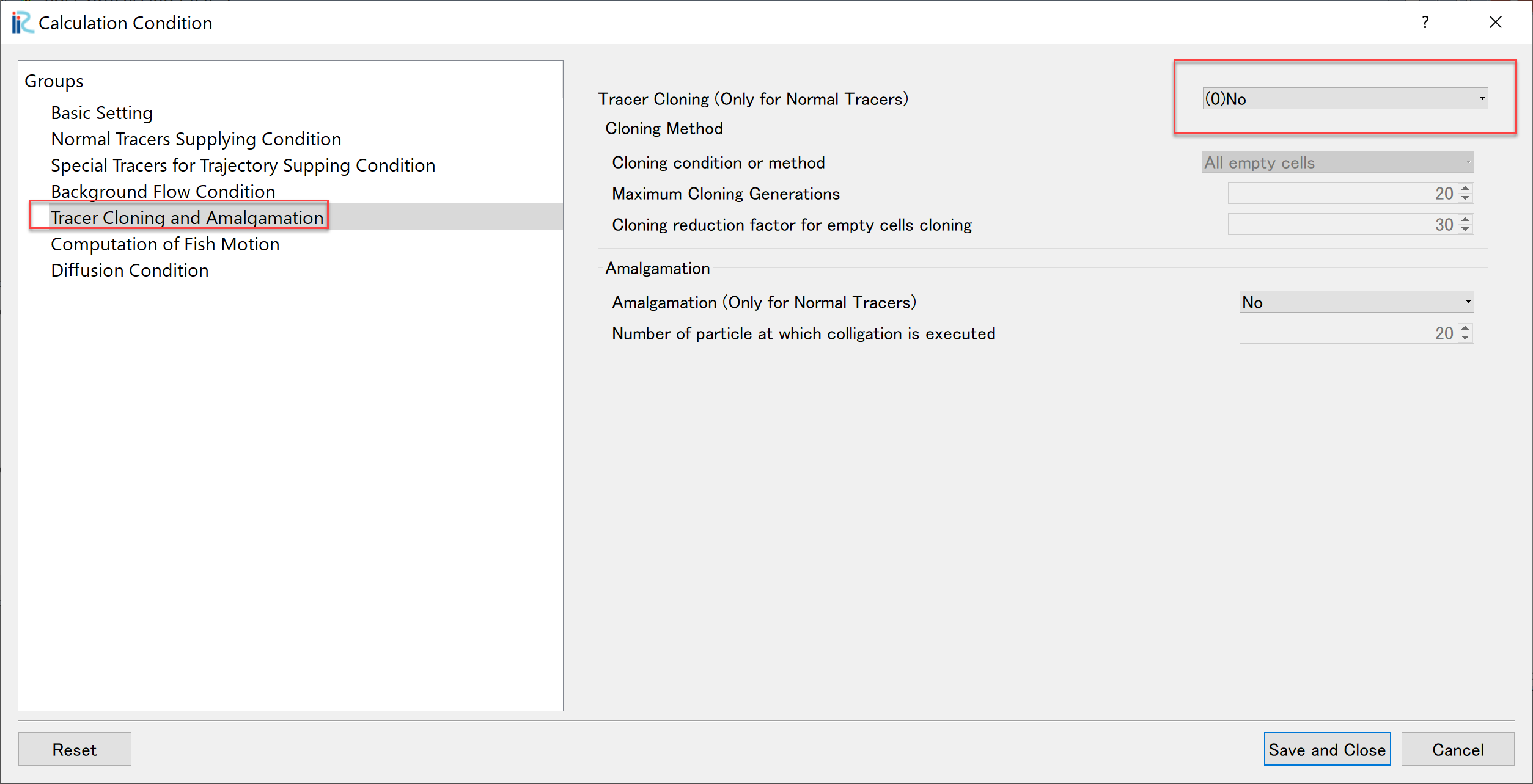
Figure 140 : Setting Condition for Fish(2)

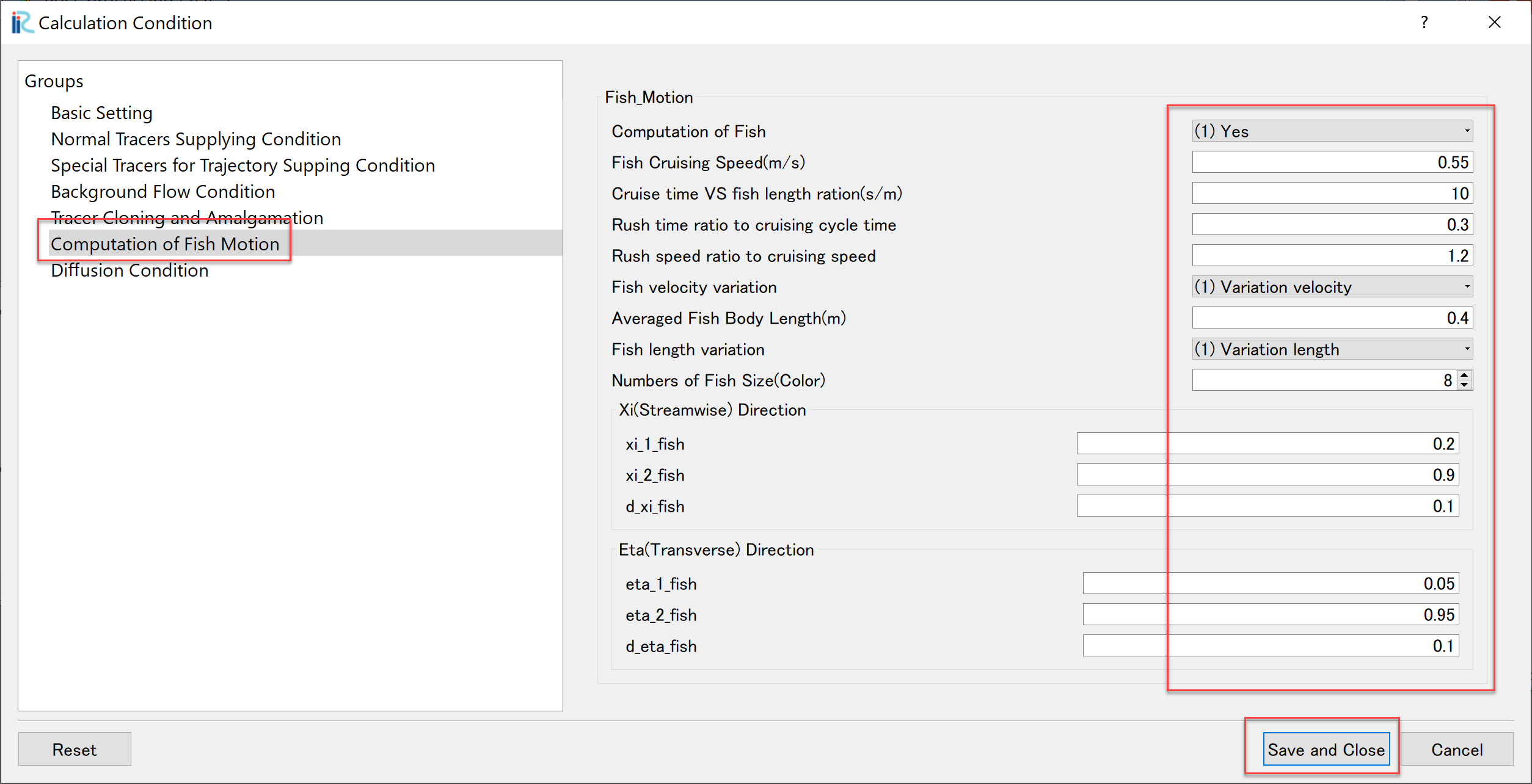
Figure 141 : Setting Condition of Fish(3)

After setting these parameters, run the solver by [Simulation]->[Run]. Once close the existing [2D Post-processing 2D window], open a new [2D Post-processing 2D window], put check mark on [Polygon]->[Fish]->[Type] as Figure 142, and select [Animation]->[Start/Stop]. Then Figure 143 is played.

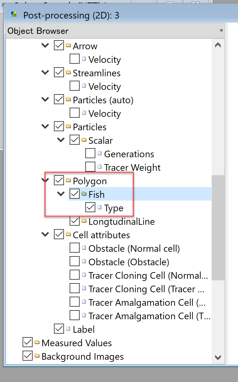
Figure 142 : Choosing Fish Animation

Figure 143 : Swimming Fish Animation

Driftwood Tracking by NaysDW2 and Visualization

In this section, driftwood tracking simulation by NaysDW2 (Nays Driftwood 3D) is shown.

Select a Solver

From the iRIC startup screen, click [Create New Project], and select [NaysDw2(Simple 2D Driftwood Tracker)] as shown in Figure 144, and press [OK].

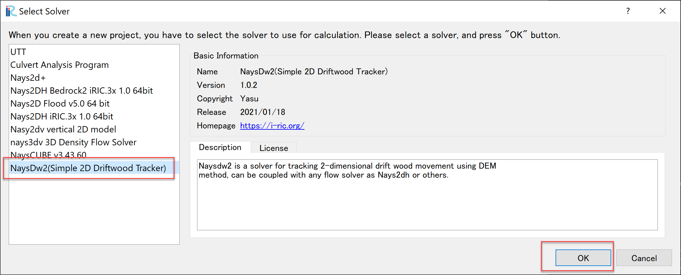
Figure 144 : Selecting [NaysDw2] (Simple 2D Driftwood Tracker)

Import Computational Grid

As shown in Figure 145, from the [Object Browser], right click [Grid(No data)], and press [Import]

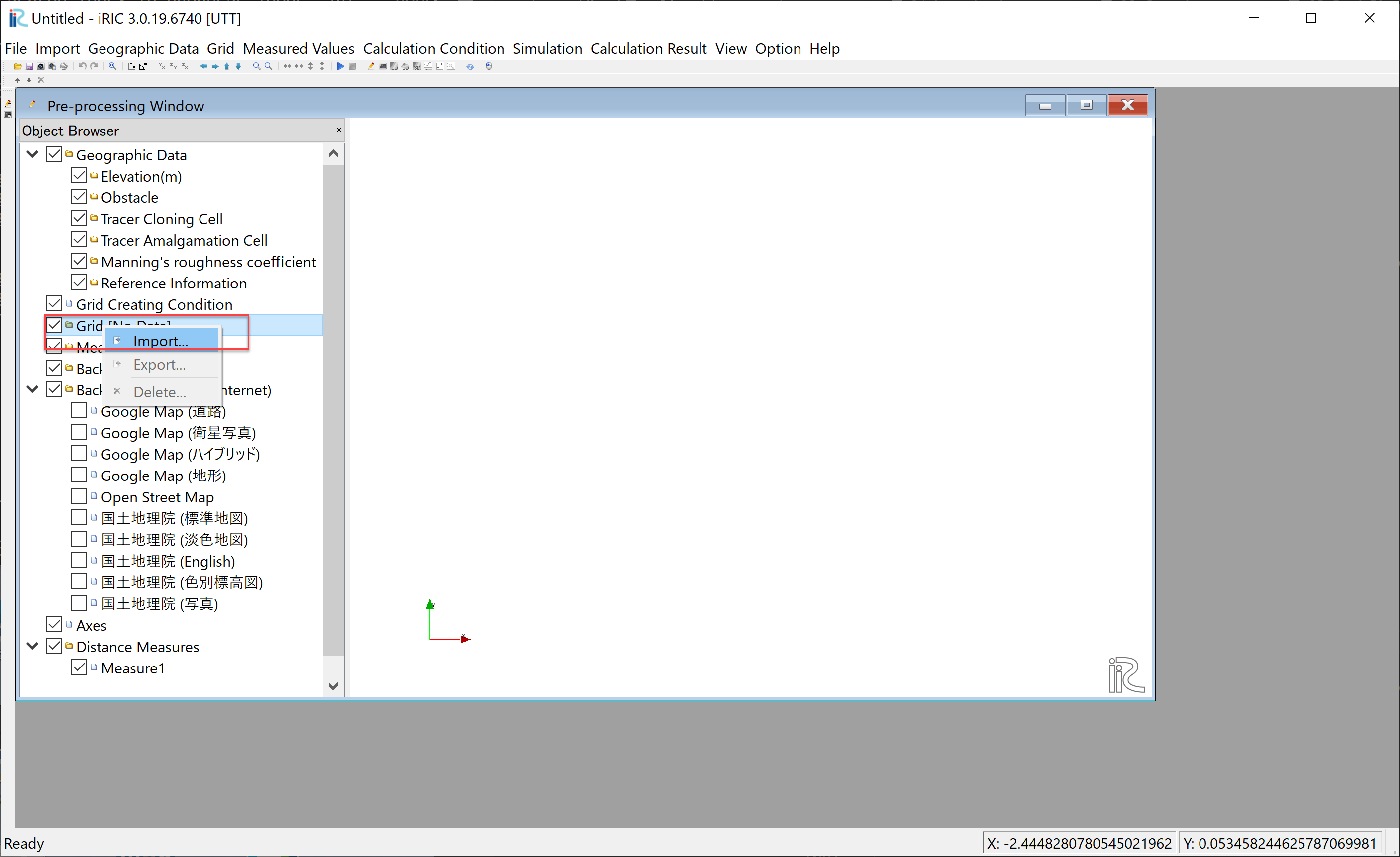
Figure 145 : [Import Grid(1)]

When the file selection window appears, select [Case1.cgn] in the [Nays2d+Flow] folder in which the computational results of the [Nays2d+] stored. (Figure 146)

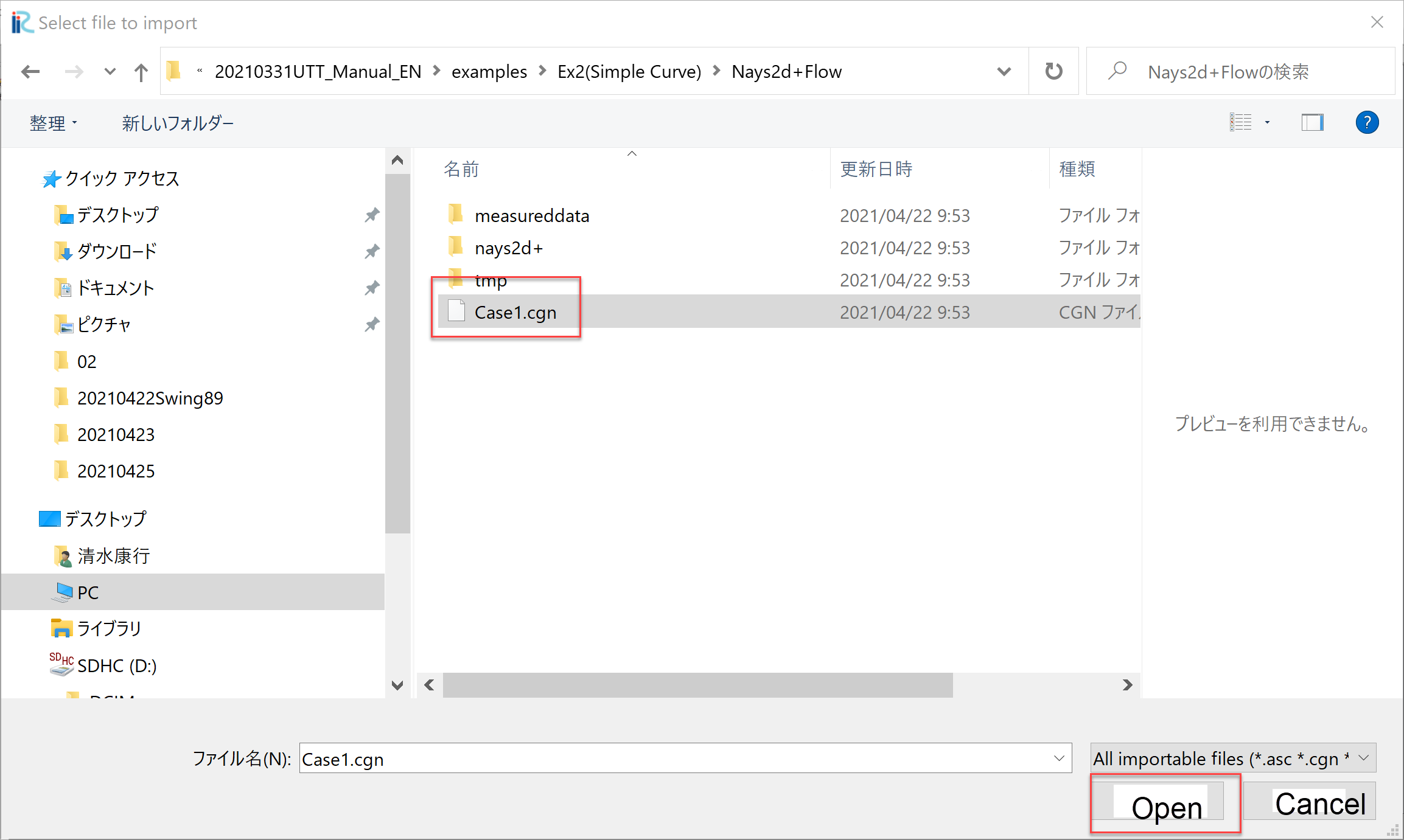
Figure 146 : [Import Grid(2)]

Neglect the waring message as Figure 102, press [Yes], and the grid importing is completed (Figure 148).

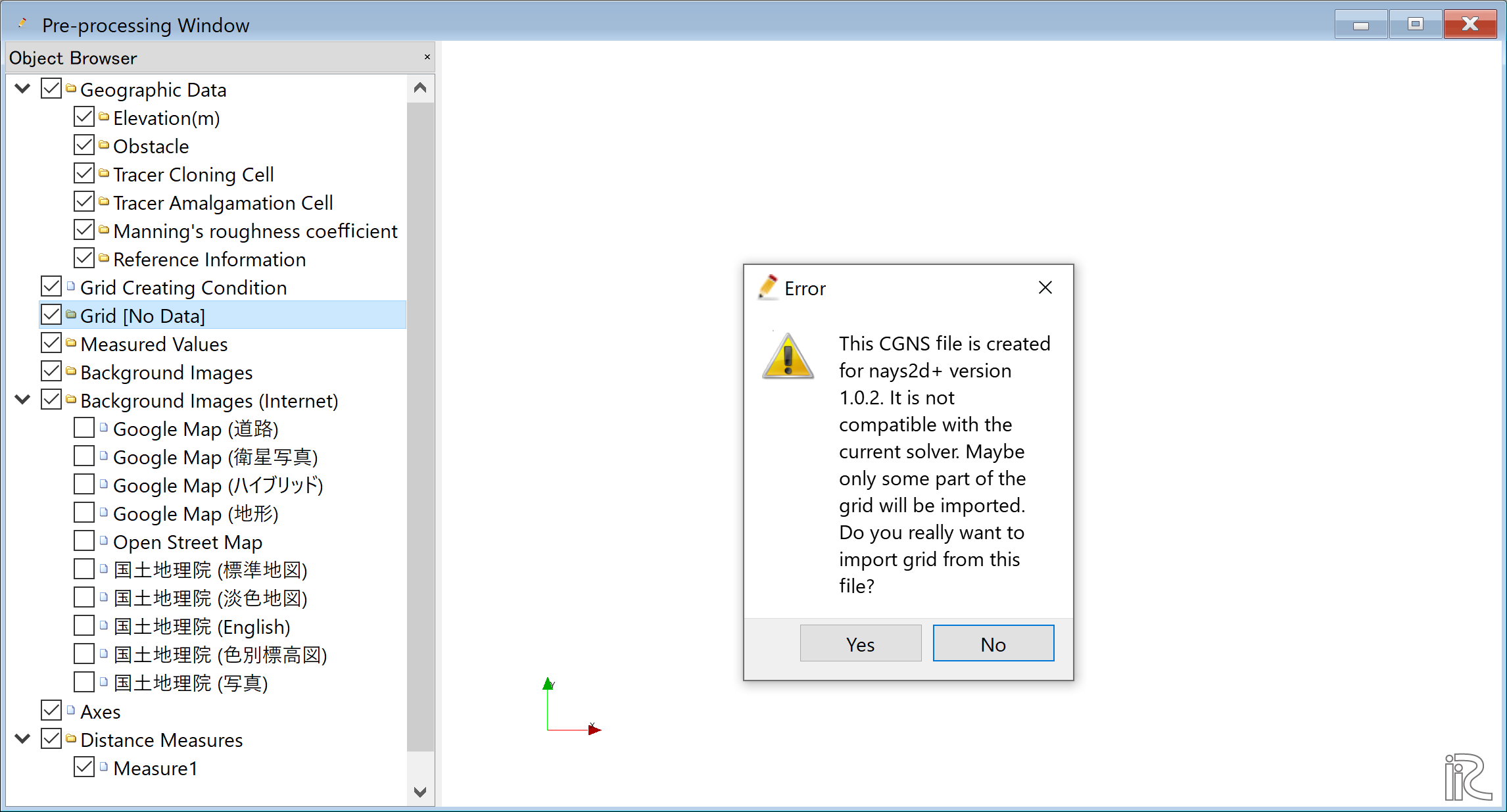
Figure 147 : [Warning Message]

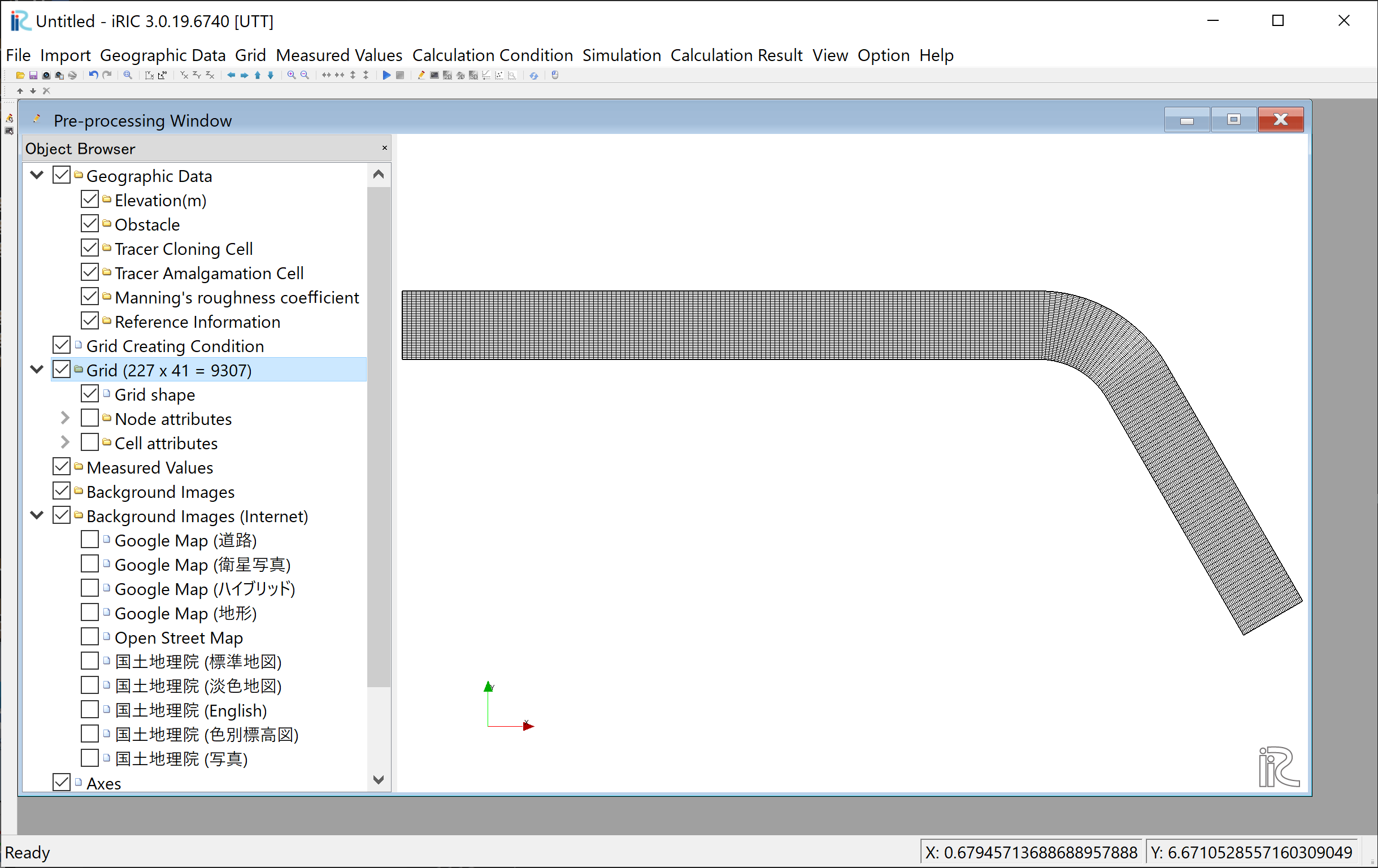
Figure 148 : [Grid Import complete]

Setting Condition

From the main menu, select [Calculation Condition]->[Setting],and set the calculation condition as follows.

In the [Calculation Condition] window, press file selection bar as Figure 149.

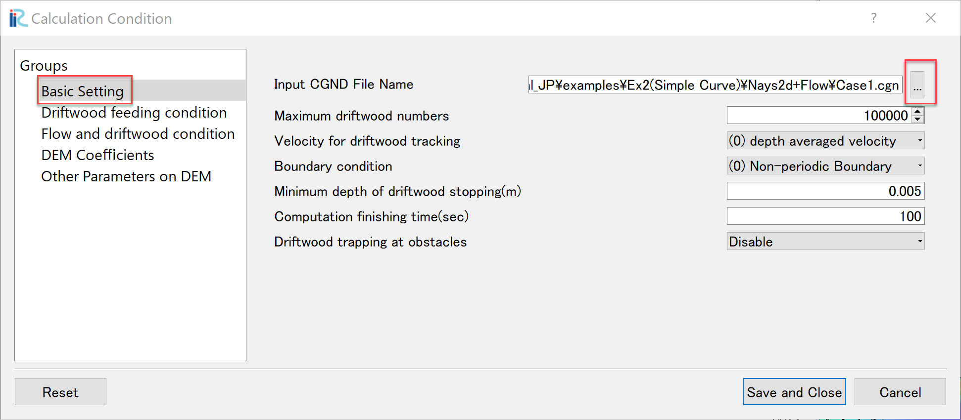
Figure 149 : Select CGNS File to Read(1)

In the [Select File] window, Figure 150, select [Case1.cgn] which contains the calculation results of the [Nays2d+] in the previous section.

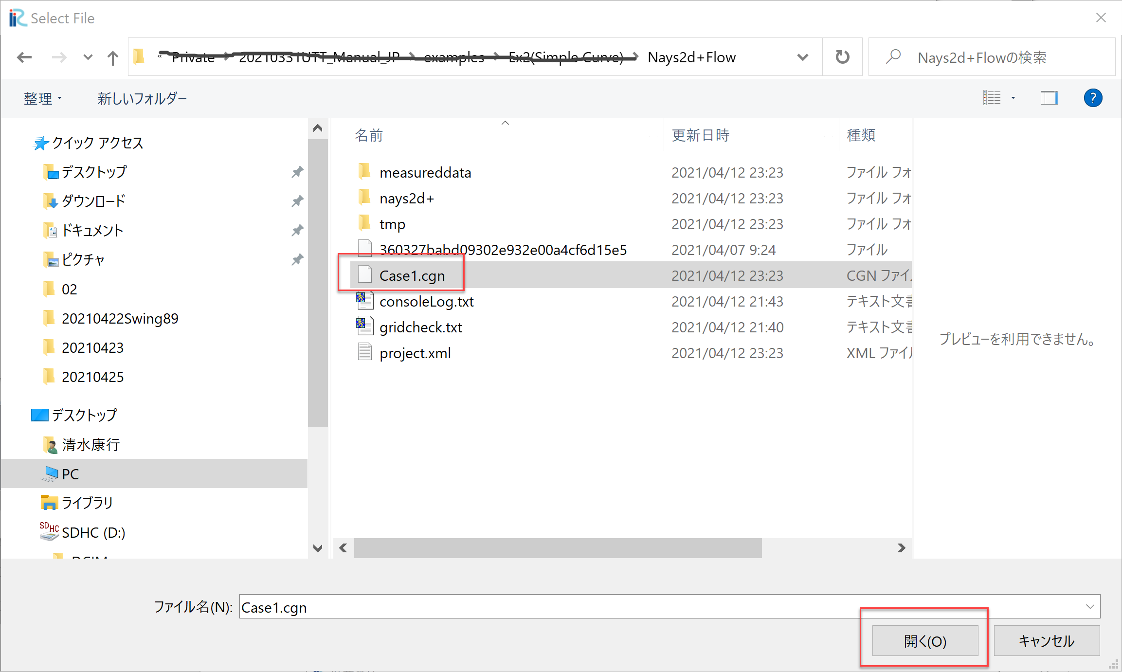
Figure 150 : Select CGNS File

Set other parameters in [Basic Setting] as Figure 151．

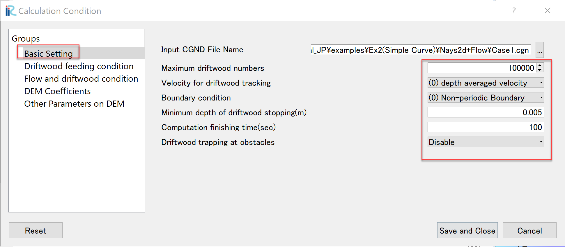
Figure 151 : Other settings in [Basic Setting]

Set parameters in [Driftwood Feeding Condition] as Figure 152．

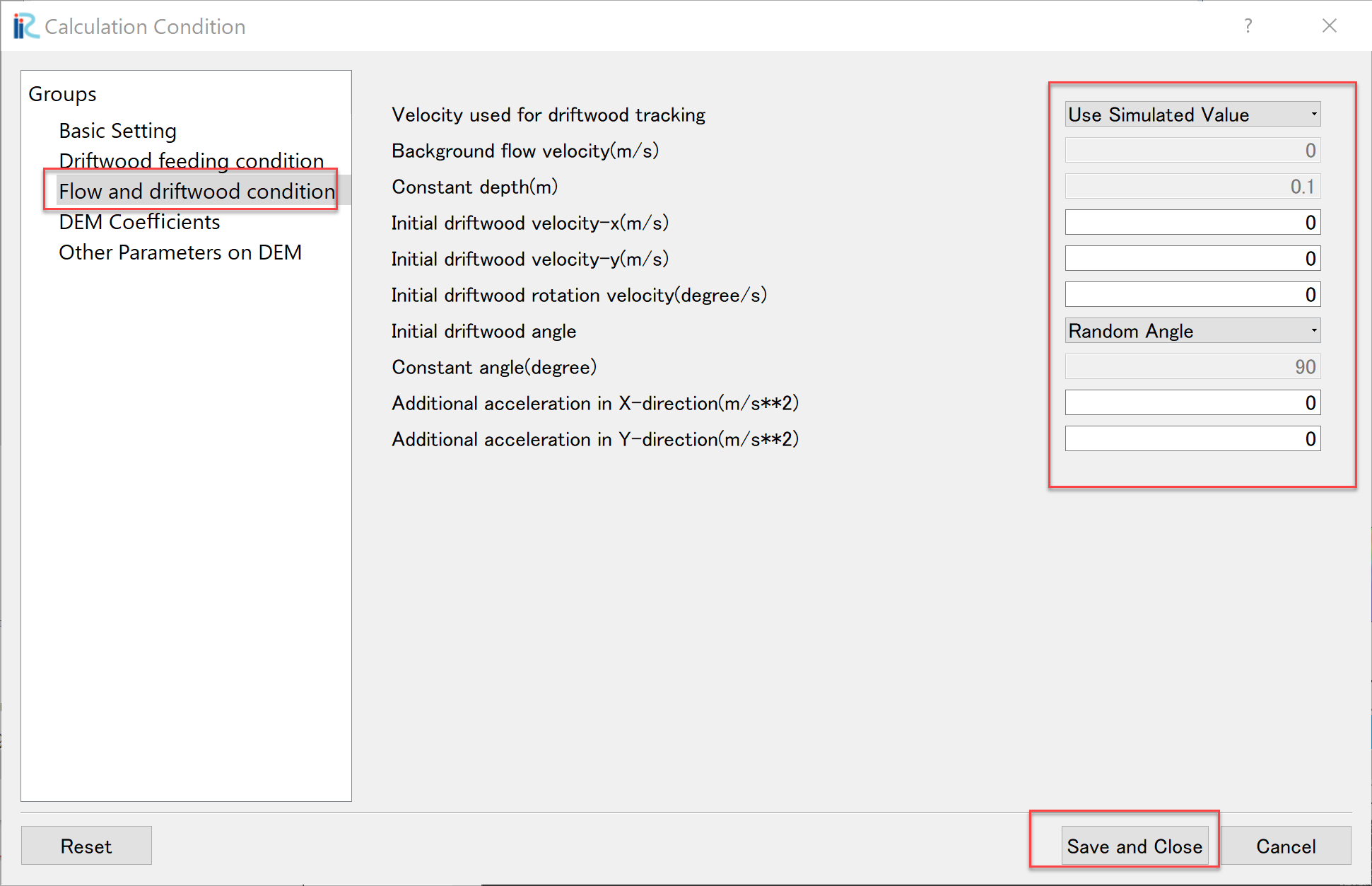
Figure 152 : [Driftwood Feeding Condition]

Set [Flow and driftwood condition] parameters as Figure 153，and press [Save and Close]．

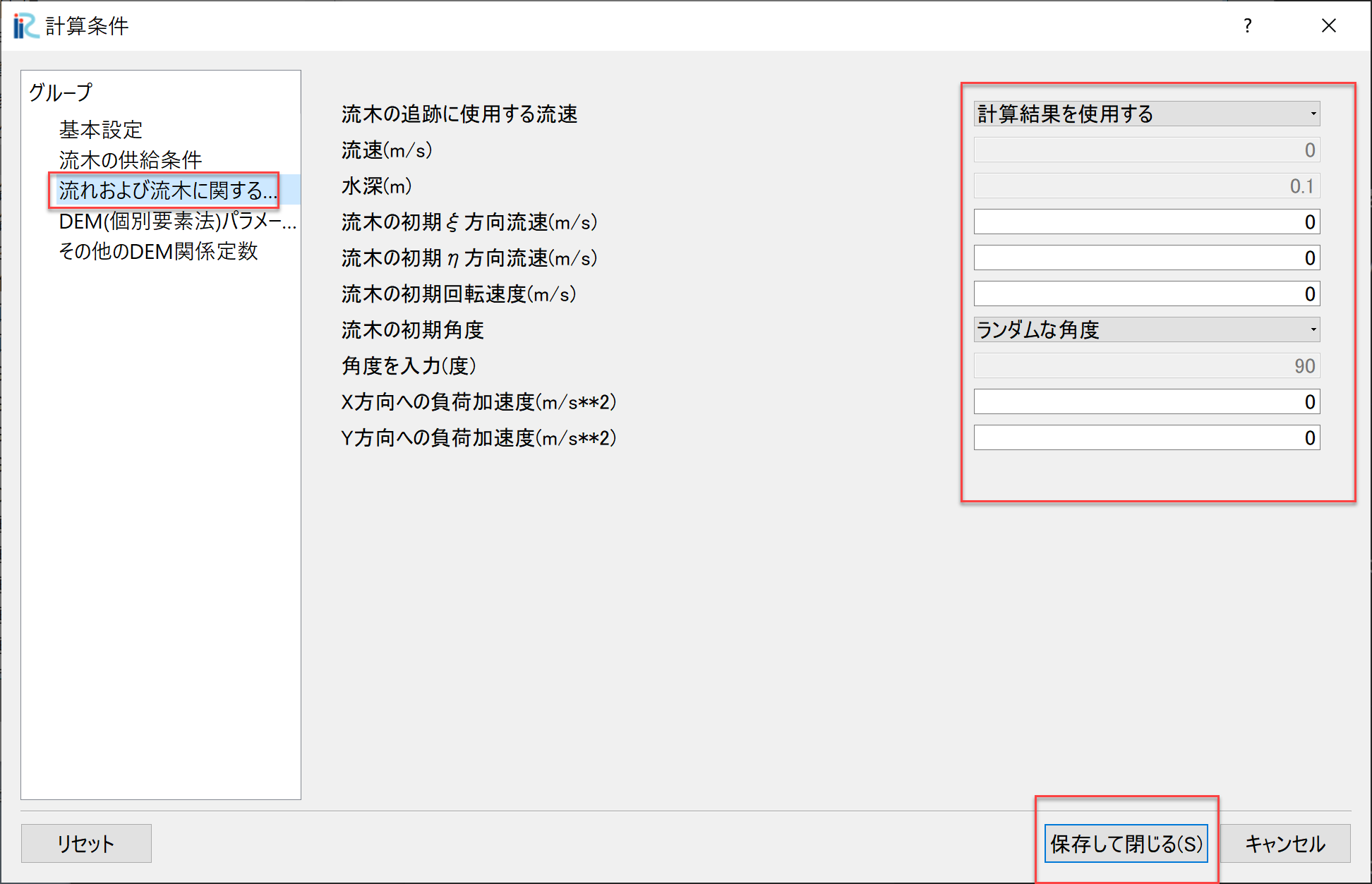
Figure 153 : [Flow and Driftwood Condition]

Run Driftwood Simulation

From the main menu, select [Simulation]->[Run] as Figure 154．

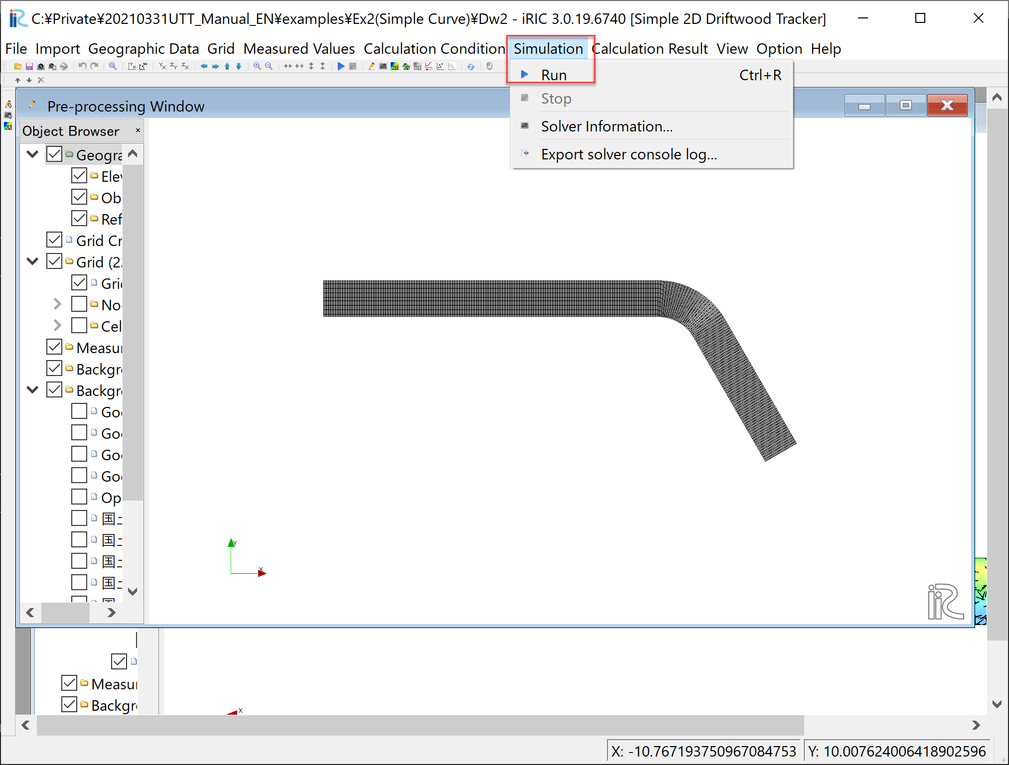
Figure 154 : [Simulation]->[Run]

When you are asked [Do you want to save?] as Figure 155, press [Yes] and save the project.

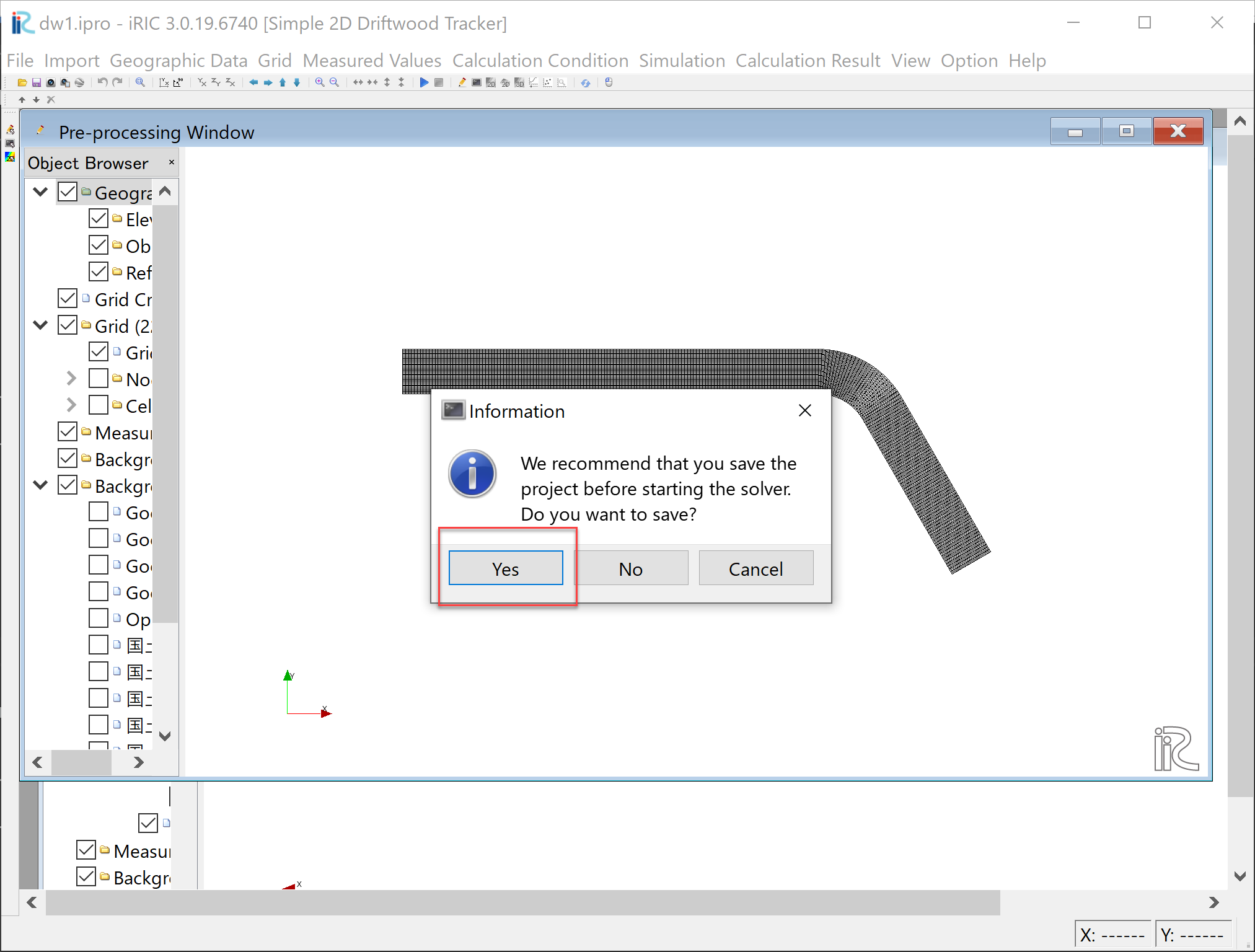
Figure 155 : [Do you want to save ?]

As Figure 156, when you are asked [How to save the project], in this example, select [Save as project], and press [OK].

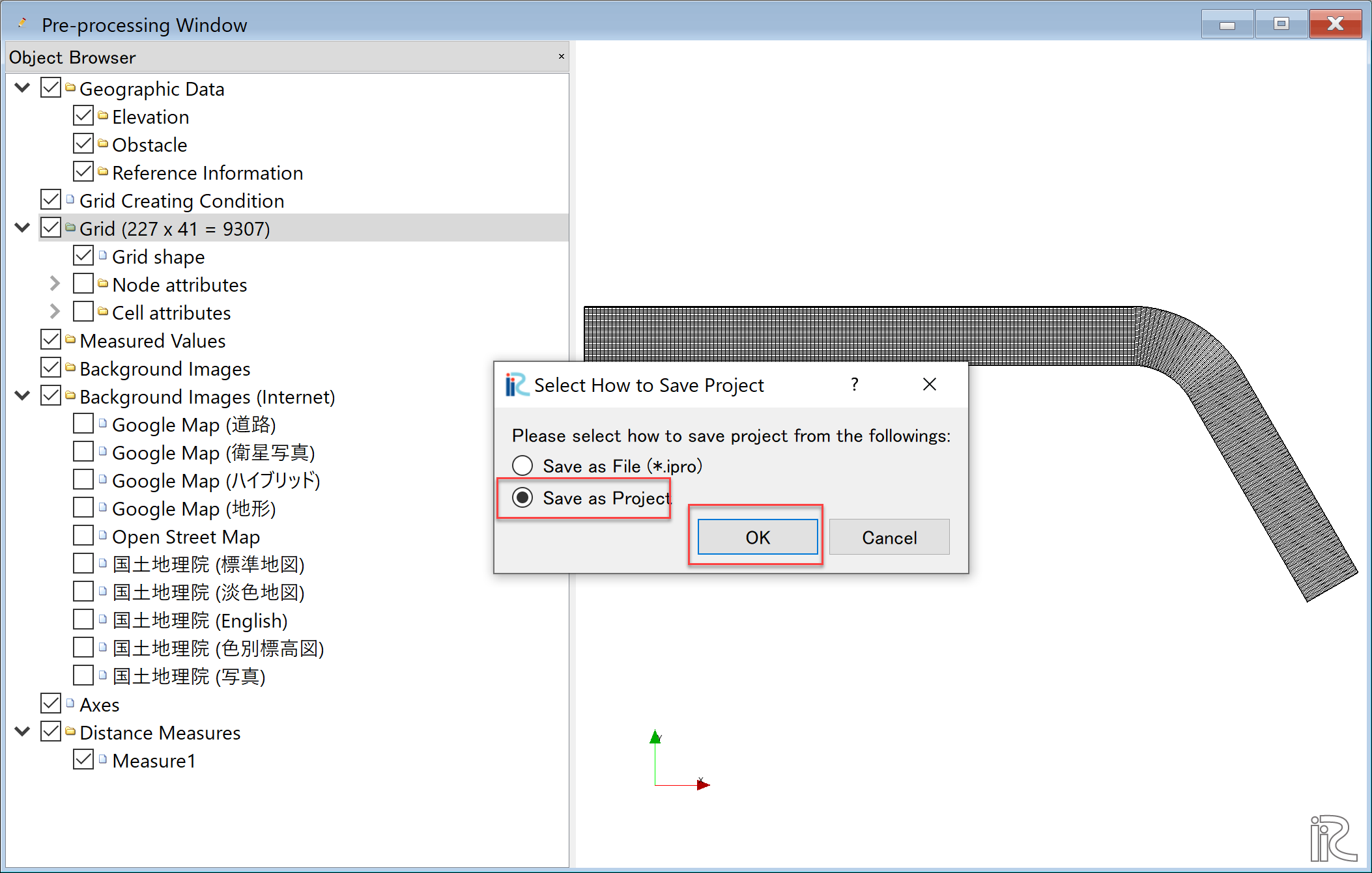
Figure 156 : [How to save project]

As Figure 157, choose an empty folder to save project, and press [Select Folder].

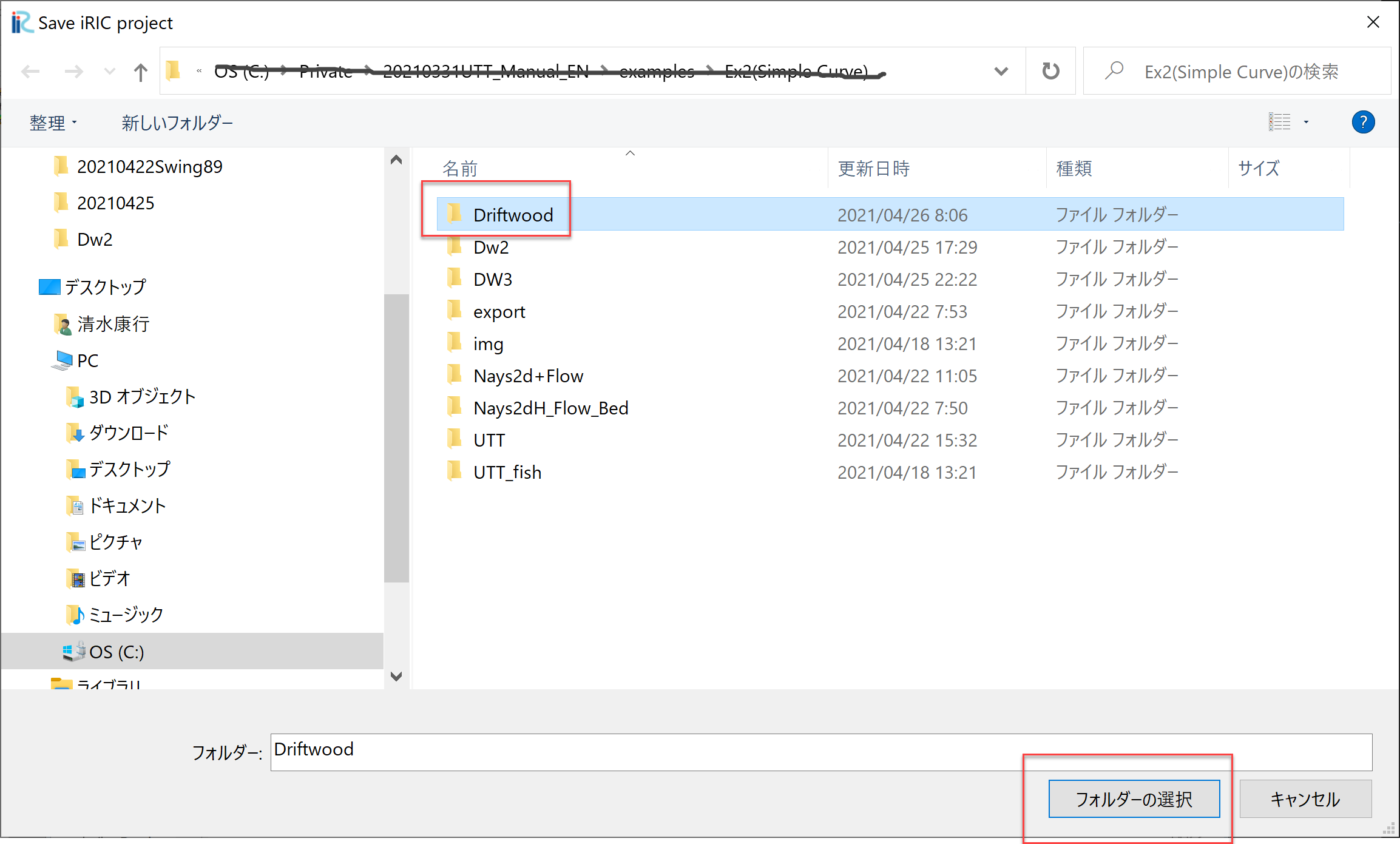
Figure 157 : Saving Project

When the calculation starts, Figure 158 is displayed, and Figure 159 is appear when the calculation ends. Then click [OK] to finish calculation.

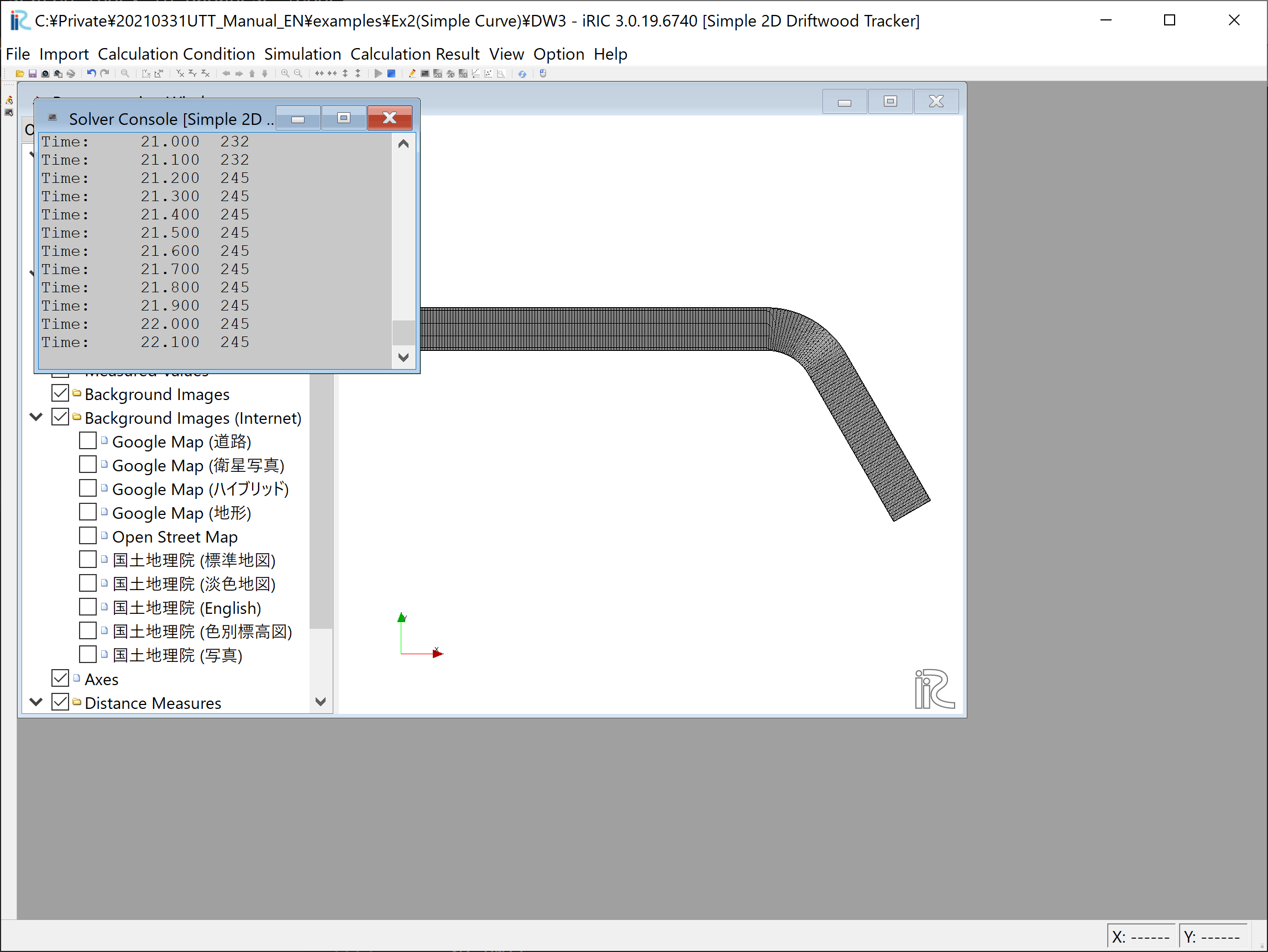
Figure 158 : Solver Running

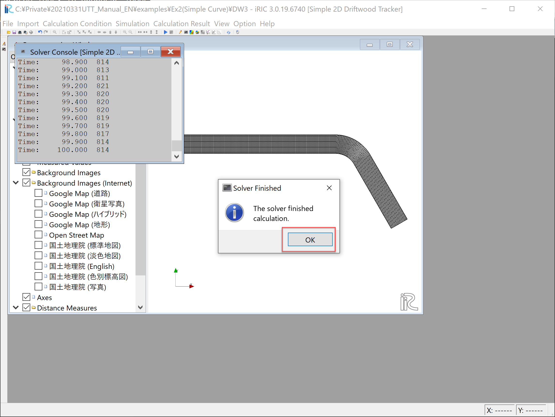
Figure 159 : Calculation finished

Visualization of driftwood motion

From the main menu, select [Calculation Result]->[Open New 2D Post-processing Window] as Figure 160.

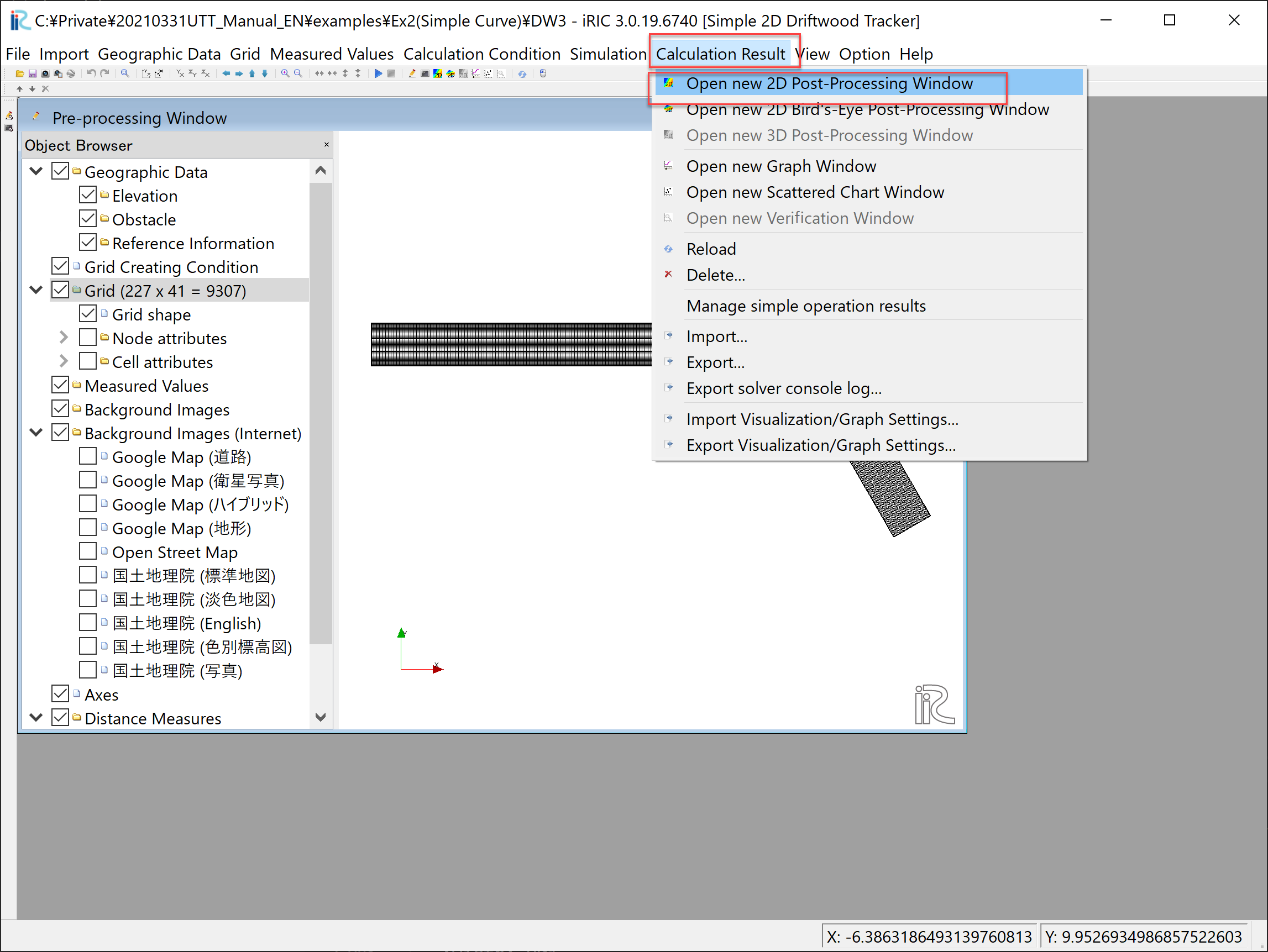
Figure 160 : Open New 2D Post-processing Window

In the [Object Browser] of Figure 161, put check marks in the boxes at [iRICZone], [Scalar(node)] and [res_Velocity(magnitude)], right click [res_Velocity(magnitude)] and choose [Property].

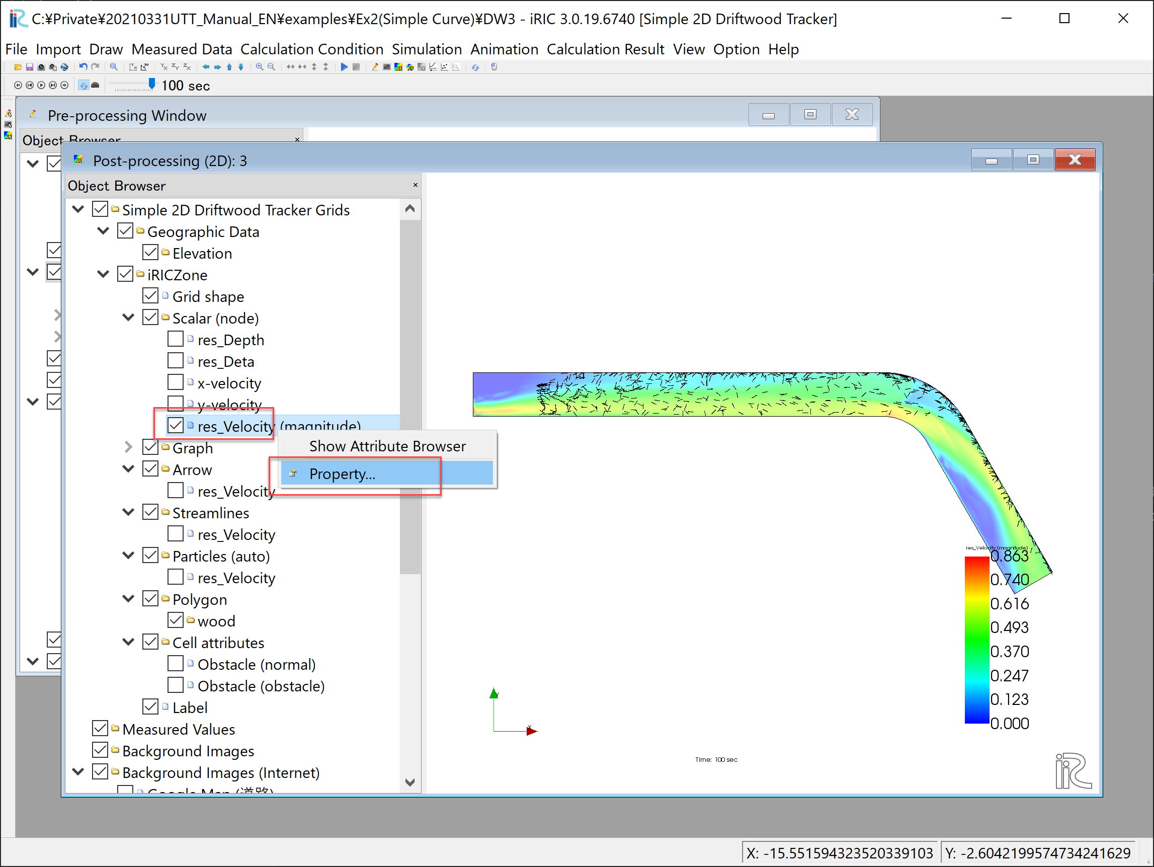
Figure 161 : Scalar Setting(1)

Set the parameters for [Scalar Settings] as Figure 162, and press [OK]．

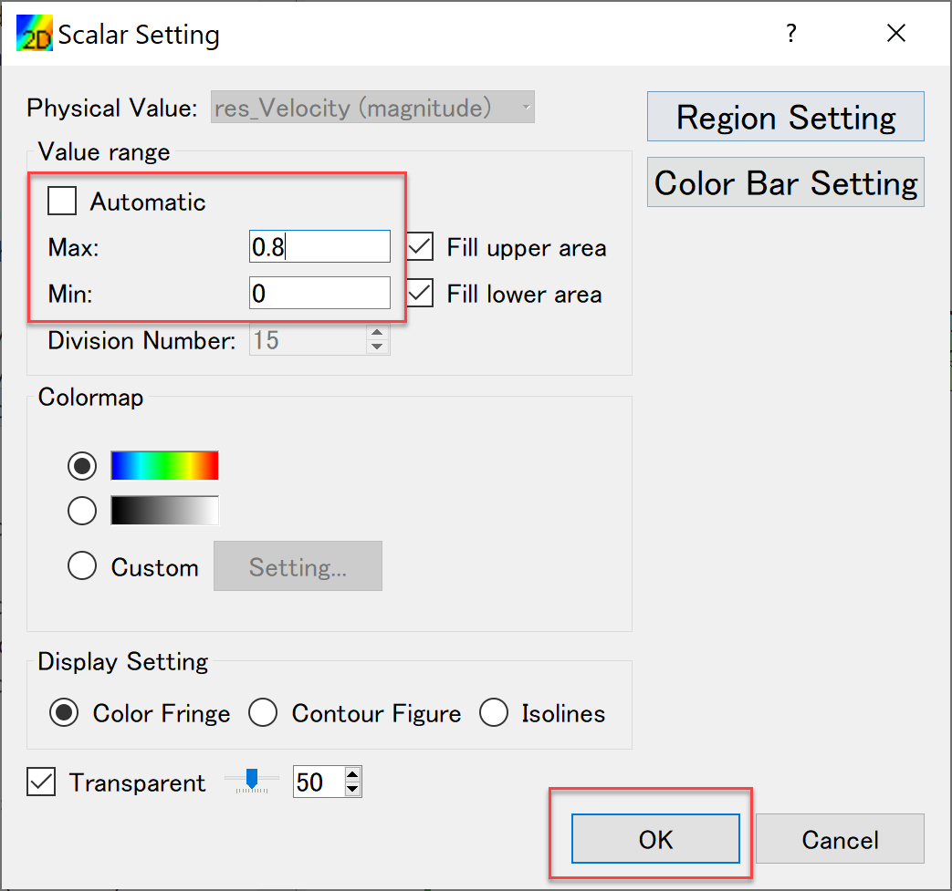
Figure 162 : Scalar Setting(2)

Press [Rotate 90° ] button twice to rotate the object 180° as Figure 163.

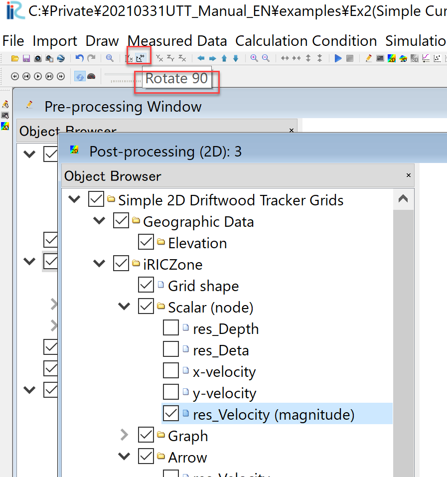
Figure 163 : 180° Rotation

Set the time bar back to zero, and select [Animation]->[Start/Stop] from the main menu bar as Figure 164, and start animation as Figure 165

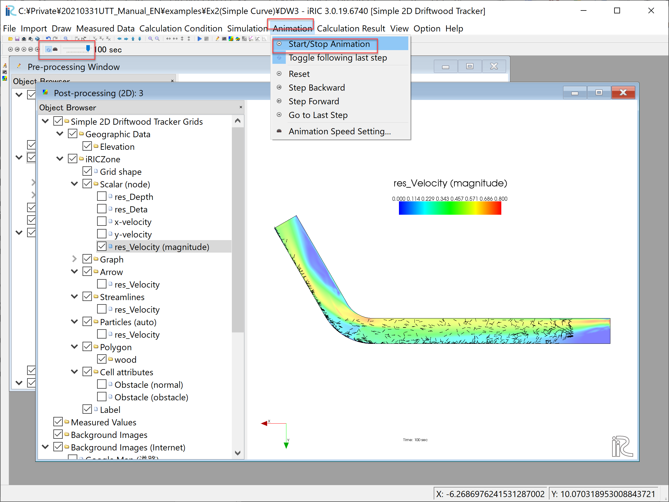
Figure 164 : Start Animation

Figure 165 : Driftwood Tracking Animation