[計算例 1]長方形水槽における自由水面の振動

Nays2dvを使って閉鎖水域(長方形の水槽)の自由水面の挙動のシミュレーションを行う。ここでは、長方形形状の水槽の水面にコサインカーブの初期擾乱を与えて、その振動の様子を観察する。

ソルバの選択

iRICの起動画面から、[新しいプロジェクト]を選ぶと表示されるソルバの選択画面で、 [Nays2dv簡単鉛直2次元密度流モデル]を選んで[OK]ボタン押すと、

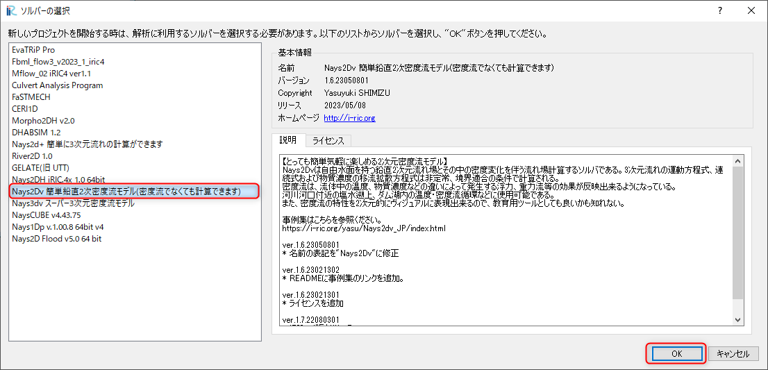
../_images/Select_solver.png — 図 4 : ソルバーの選択

「無題- iRIC 3.x.xxxx [Nays2dv簡単鉛直2次元密度流モデル]」と書かれた Windowが現れる。

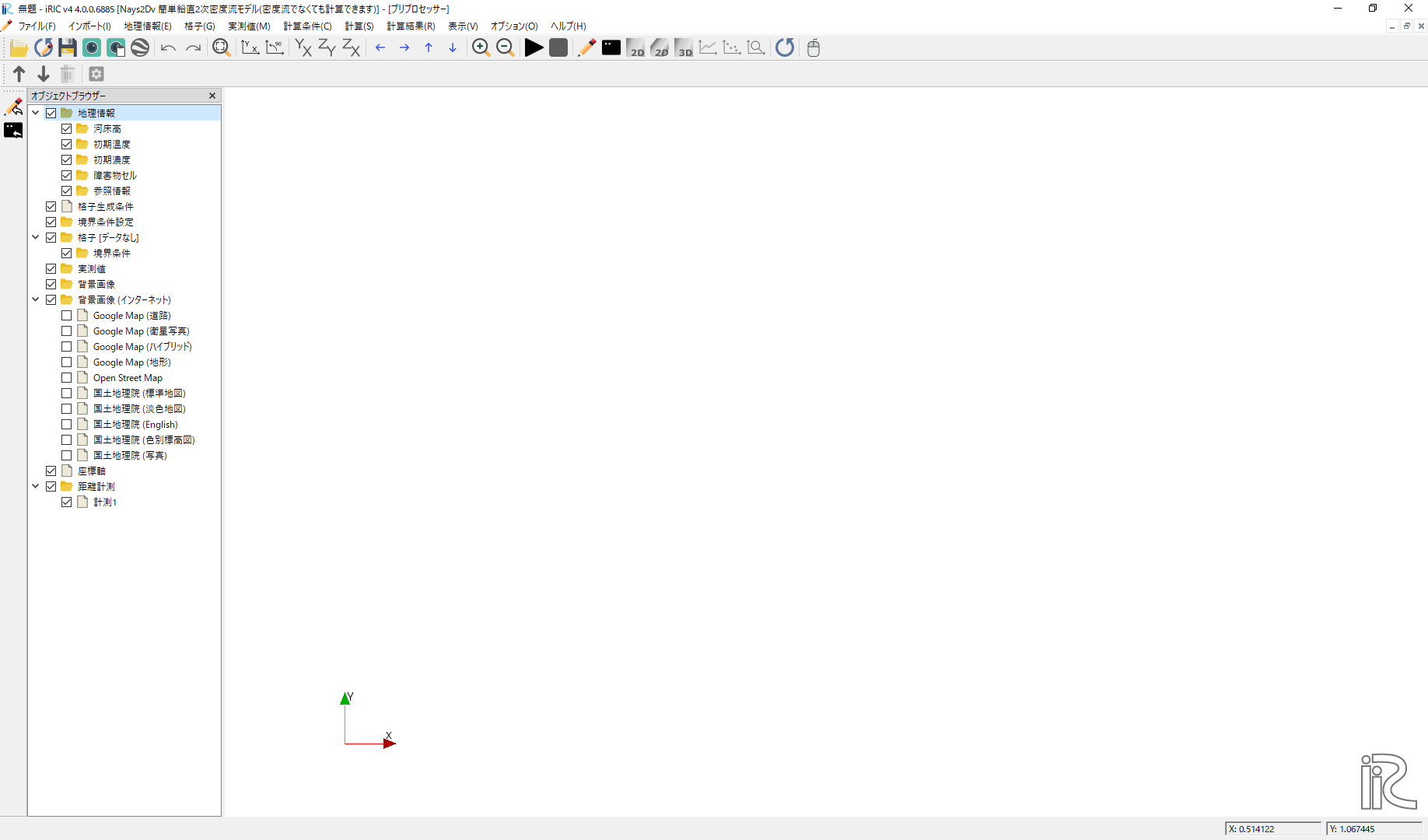
../_images/mudai.png — 図 5 : 無題

計算格子の作成はNays2dv専用の格子生成ツールを用いる。図 5 のウィンドウで、[格子]→[格子生成アルゴリズムの選択]から現れる、「格子生成アルゴリズムの選択」ウィンドウで[Nays2dv用格子生成ツール]を選んで[OK]を押す。

../_images/koushi_sentaku.png — 図 6 : 格子生成アルゴリズムの選択

計算格子の作成

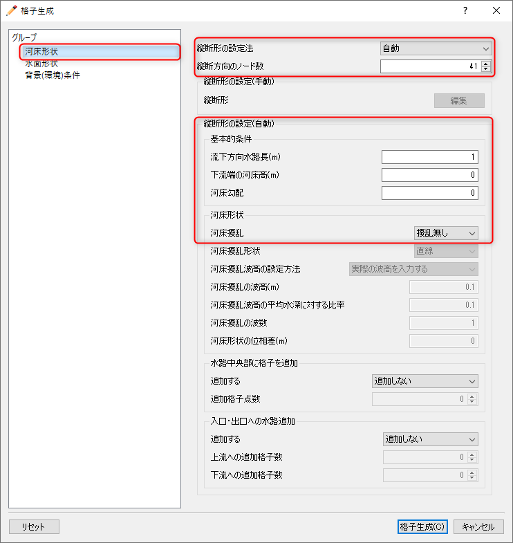
../_images/koushi_1.png — 図 7 :格子生成(計算領域)形状

図 7 の画面で、[グループ]で[河床形状]を選び。「縦断方向のセル数」を[41]、「流下方向水路長(m)」を[10]、「下流端の河床高(m)」を[-1]、「河床勾配」を[0]、「河床形状」を[擾乱無し]とする。入力が終わったら「水面形」のグループへ移動する。

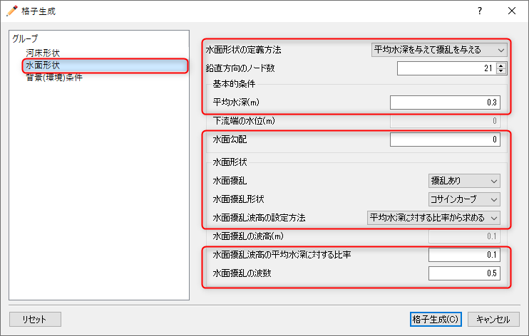
../_images/koushi_2.png — 図 8 :格子生成(計算領域)形状

図 8 の画面で、「水面形の定義方法」を[平均水深を与えて擾乱を与える]、「平均水深(m)」を[0.3]、「鉛直方向のノード数」を[21]、水面勾配」を[0]、「水面擾乱」を [擾乱あり]、「水面擾乱形」を[コサインカーブ]、「擾乱の波高(m)」を[０.1]、擾乱波数を[0.5]として、最後に[格子生成]ボタンを押す。

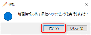
../_images/koushi_3.png — 図 9 :確認(マッピング)

すると、図 9 確認ウィンドウが現れるので、[はい(Y)]を押すと格子が生成され、下図図 10 が表示される。

../_images/koushi_4.png — 図 10 :格子生成完了

計算条件の設定

次に計算条件の設定を行う。メニューバーから「計算条件」→「設定」を選ぶと、計算条件設定ウィンドウ図 11 が表示される。

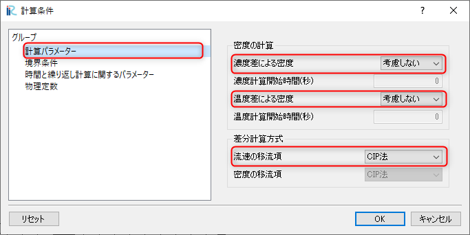
../_images/jouken_1.png — 図 11 :計算パラメータ

密度流の計算ではないので「密度の計算」は[考慮しない]、「温度差による密度」も[考慮しない]、「差分計算方法」の「流速の移流項」は[CIP法]とする。

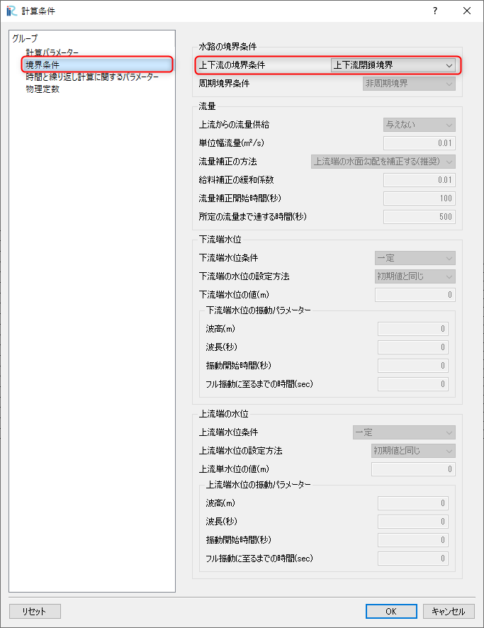
../_images/jouken_2.png — 図 12 :初期条件と境界条件

次に、「境界条件」図 12 に移る。閉鎖水路の水面振動なので、「上下流の境界条件」は [上下流閉鎖条件]を選び、「時間と繰り返し計算に関するパラメーター」に移動する。

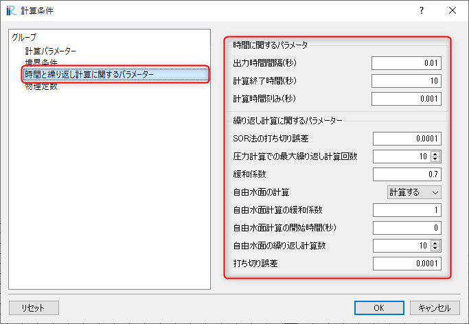
../_images/jouken_3.png — 図 13 :時間と繰り返し計算に関するパラメーター

「時間および繰り返し計算に関するパラメーター」図 13 図に示したようなパラメータを設定する。なお、自由水面振動の計算なので、「自由水面の計算」は必ず[計算する]にしておく必要がある。

設定が終わったら[保存して閉じる]を押す。

計算の実行

図 14 の画面で、メニューバーから[計算]→[実行]を選ぶと、図 15 の画面が現れるので、「はい(Y)」を選んで、計算条件を保存しておく。保存はipro形式または、プロジェクト形式を選択する。

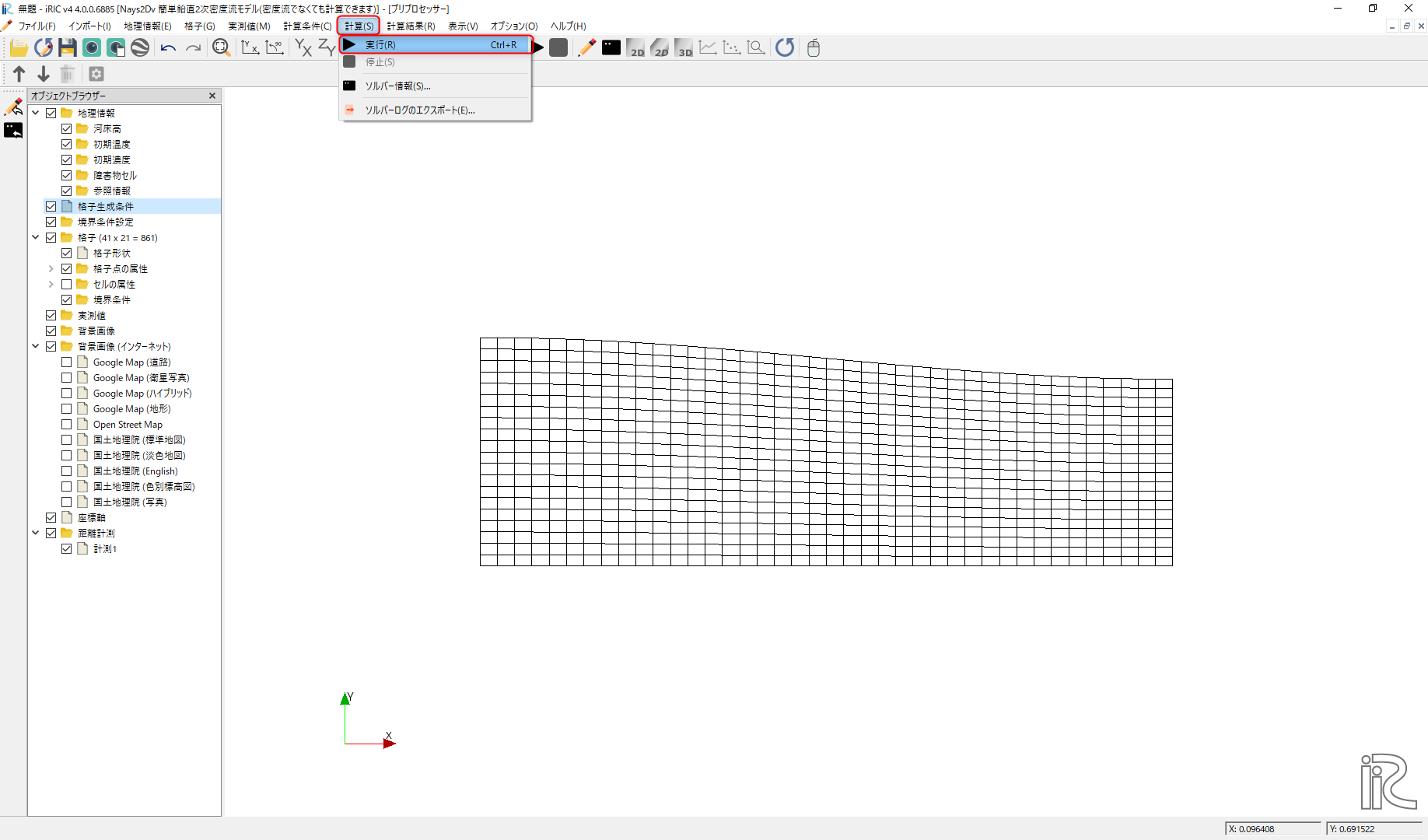
../_images/jikko1.png — 図 14 :計算の実行(1)

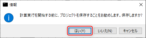
../_images/jikko2.png — 図 15 :保存しますか？

保存が終了すると、図 16 の画面が現れ、計算が始まる。

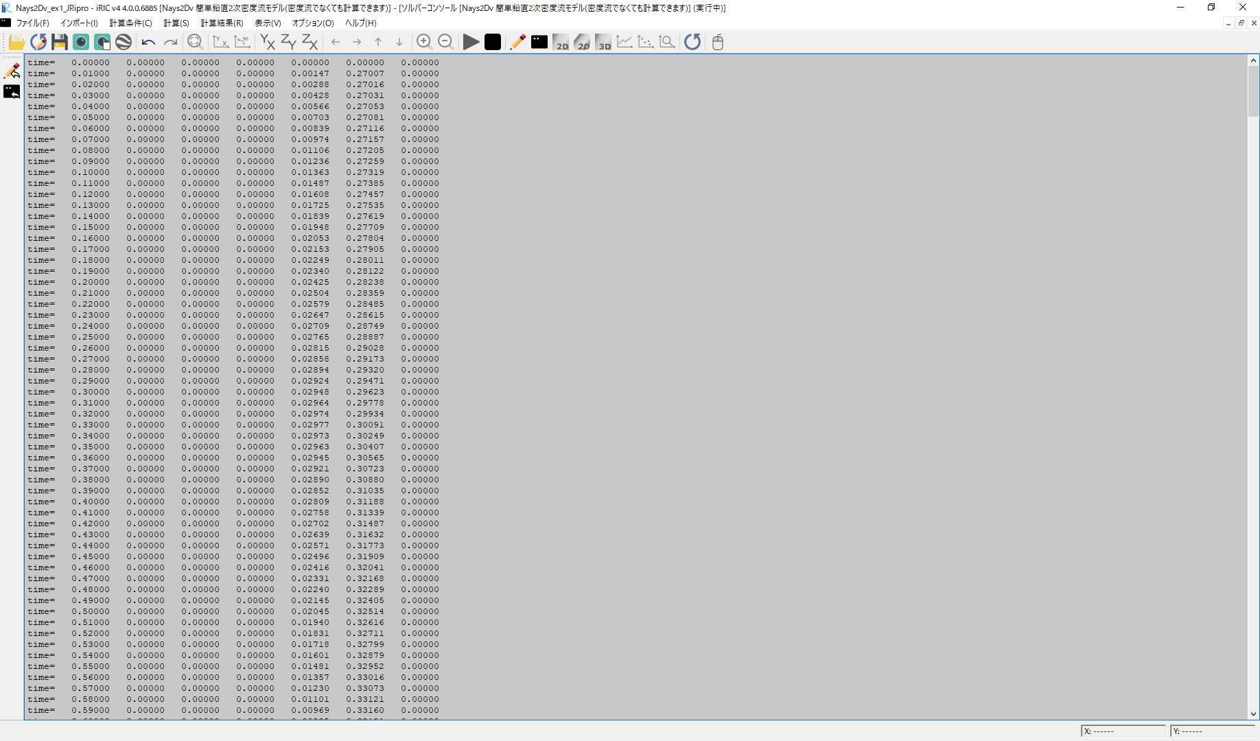
../_images/jikko3.png — 図 16 :計算実行中

計算が終了すると、図 17 の画面が現るの[OK]を押す。

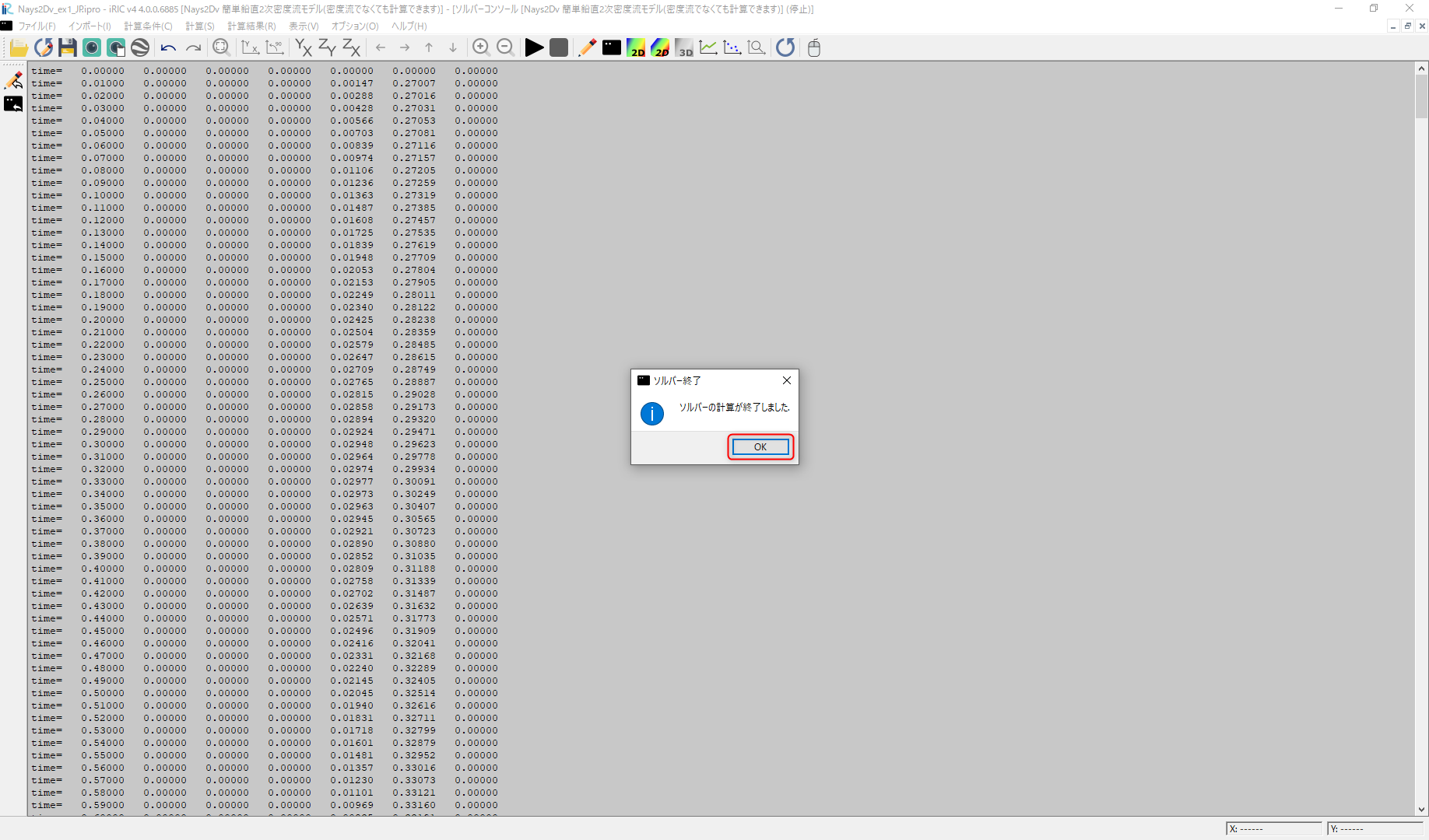
../_images/jikko4.png — 図 17 :計算終了

計算結果の表示

計算の終了後、図 18 の画面で[計算結果]→[新しい可視化ウィンドウ(2D)を開く]を選ぶことによって、可視化ウィンドウ図 19 が現れる。

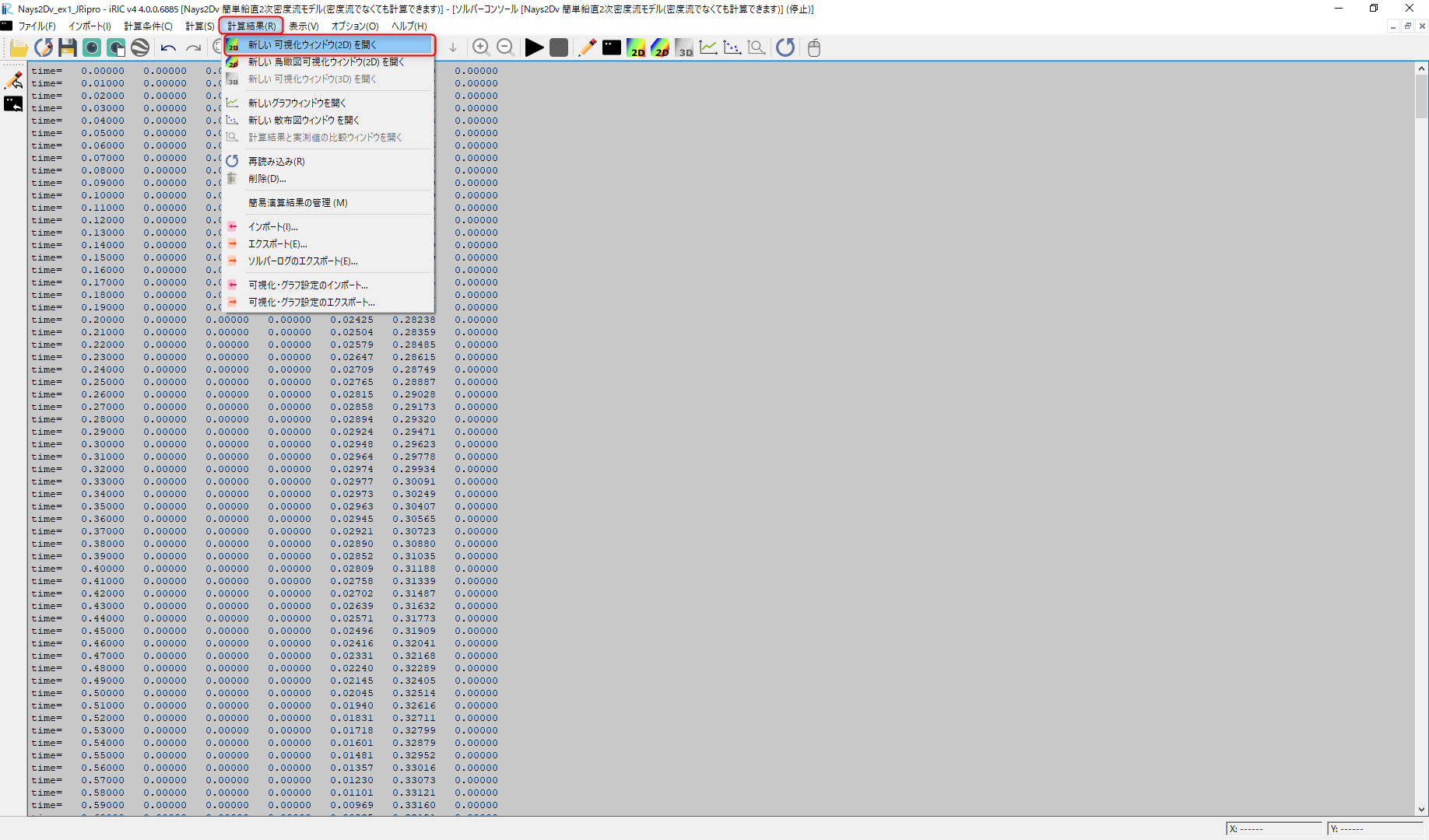
../_images/kekka_1.png — 図 18 : 計算結果の表示(1)

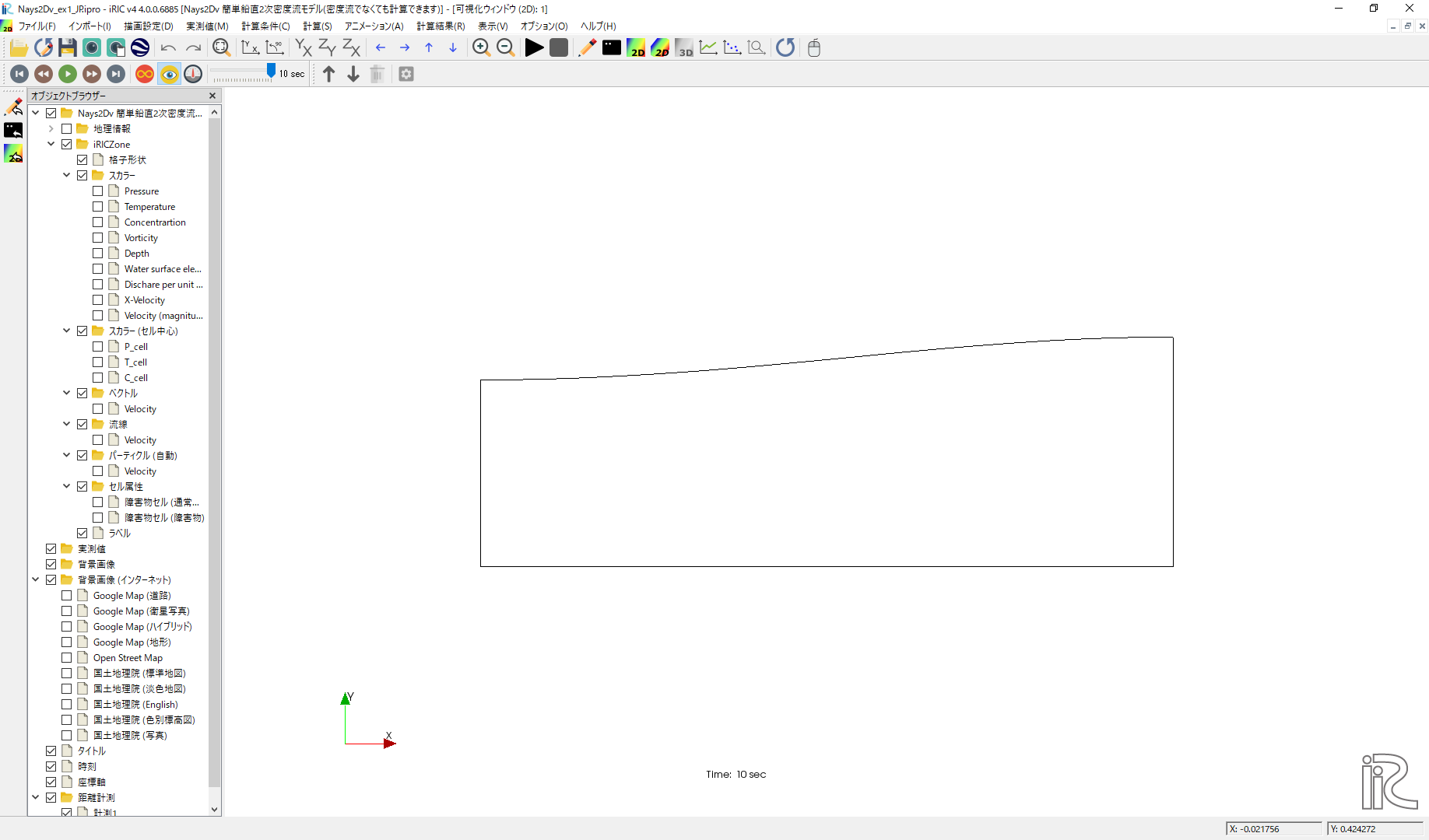
../_images/kekka_2.png — 図 19 : 計算結果の表示(2)

図 19 が現れた段階で、図 20 に示す[アニメーション]→[開始/停止]を押すことにより水面の振動アニメーションの開始と停止が可能となる。のアニメーションの開始と停止はツールバーの[開始/停止]ボタンからでも可能である。

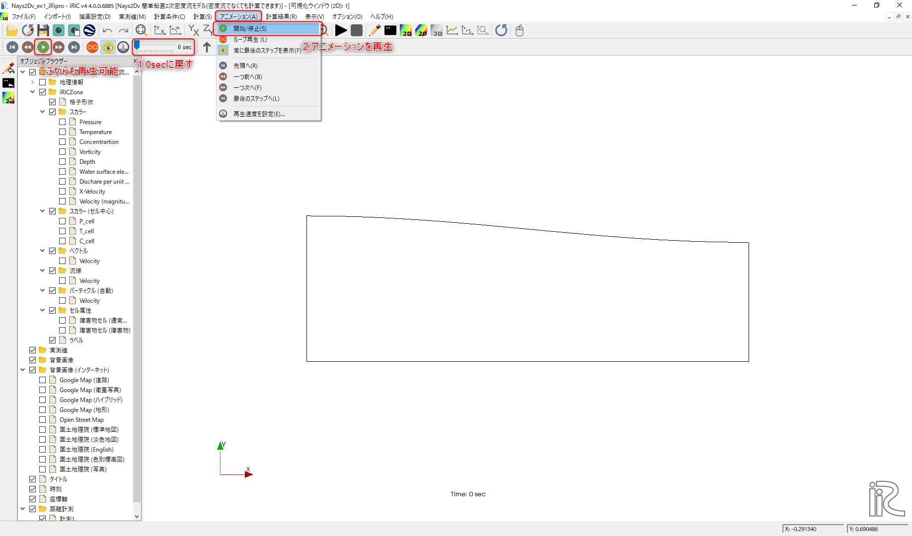
../_images/kekka_3.png — 図 20 : 動画の表示

このとき、マウスのセンターダイヤを回すことにより、拡大・縮小が可能となっている。

ベクトルの表示

オブジェクトブラウザーで、[ベクトル]を右クリックして、[プロパティ]をクリックすると、「ベクトル設定」ウィンドウ図 21 が現れる。

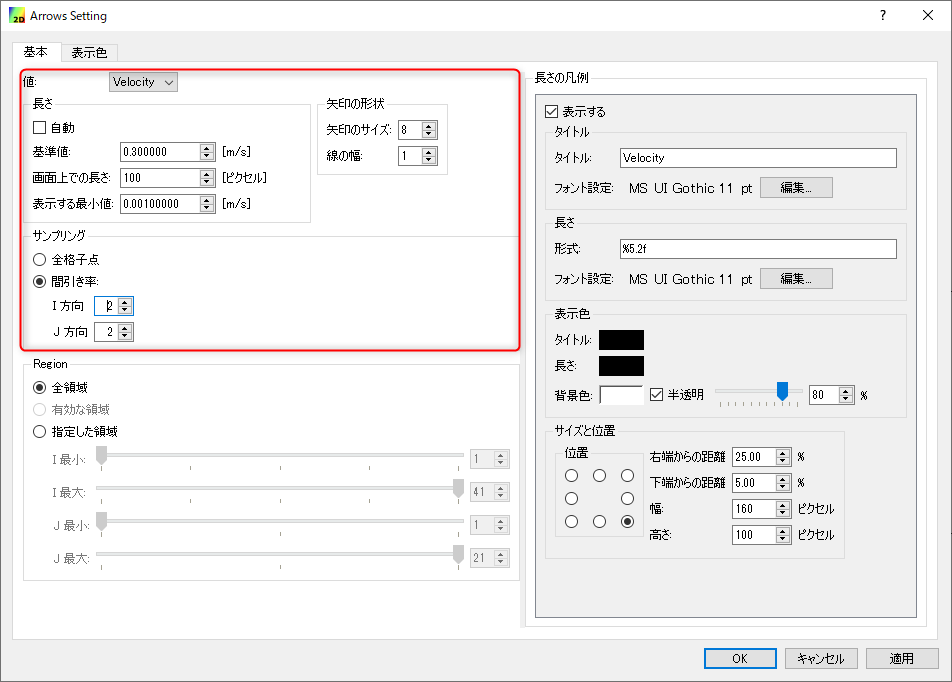
../_images/kekka_4.png — 図 21 : ベクトルの設定

図 21 の赤囲の部分の設定をして、[OK]をクリックする。 [アニメーション]→[開始/停止]ボタンで、図 22 のアニメーションが表示される。

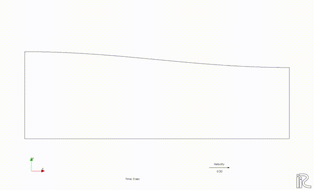
../_images/kekka_5.gif — 図 22 : ベクトルのアニメーション

圧力の表示

オブジェクトブラウザーで、図 23 [スカラー][Pressure]に☑チェックを付けて、ここを右クリックして、[プロパティ]を選ぶと、「コンター設定」ウィンドウ図 24 が現れる。ここで、赤枠の設定をして[OK]を押すと図 25 が表示される。

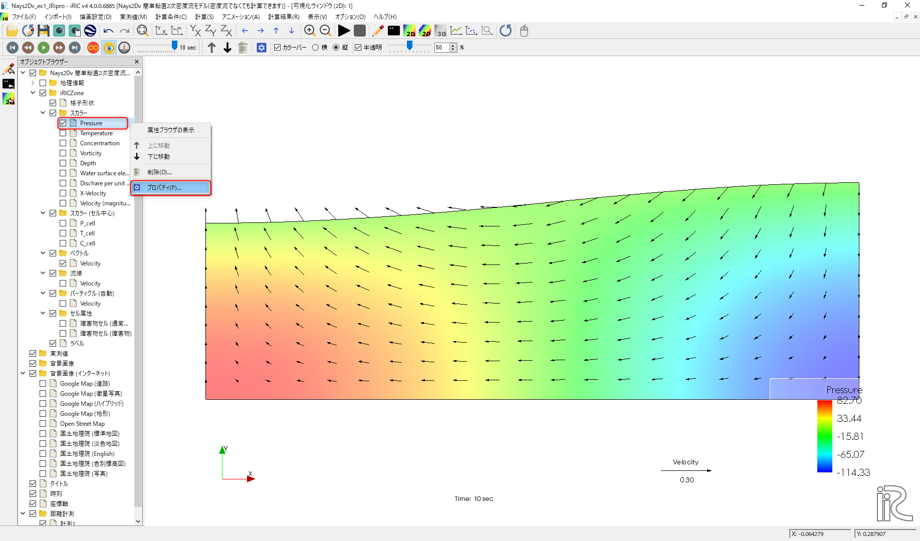
../_images/kekka_7.png — 図 23 : 圧力表示

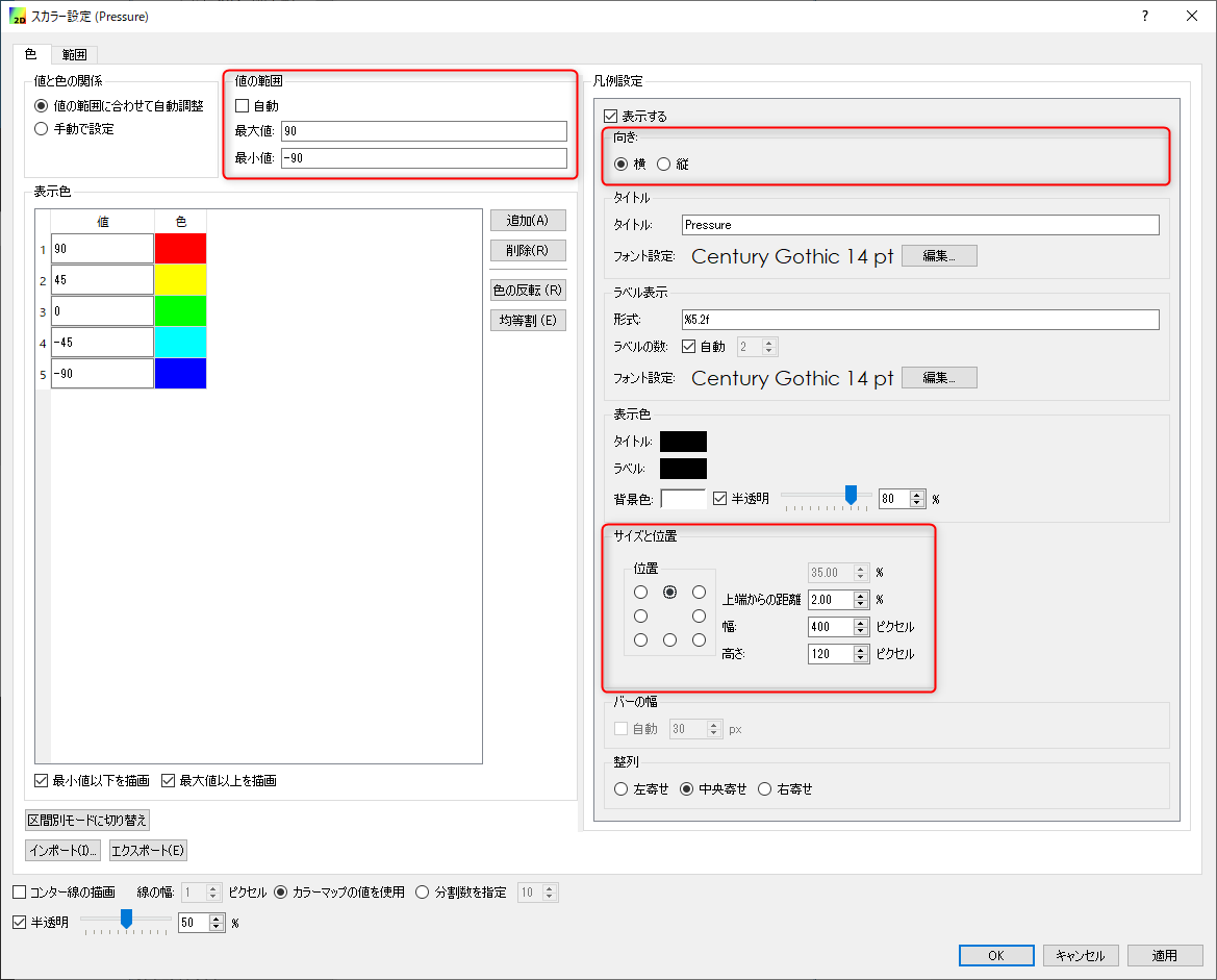
../_images/kekka_8.png — 図 24 : 圧力コンターの設定

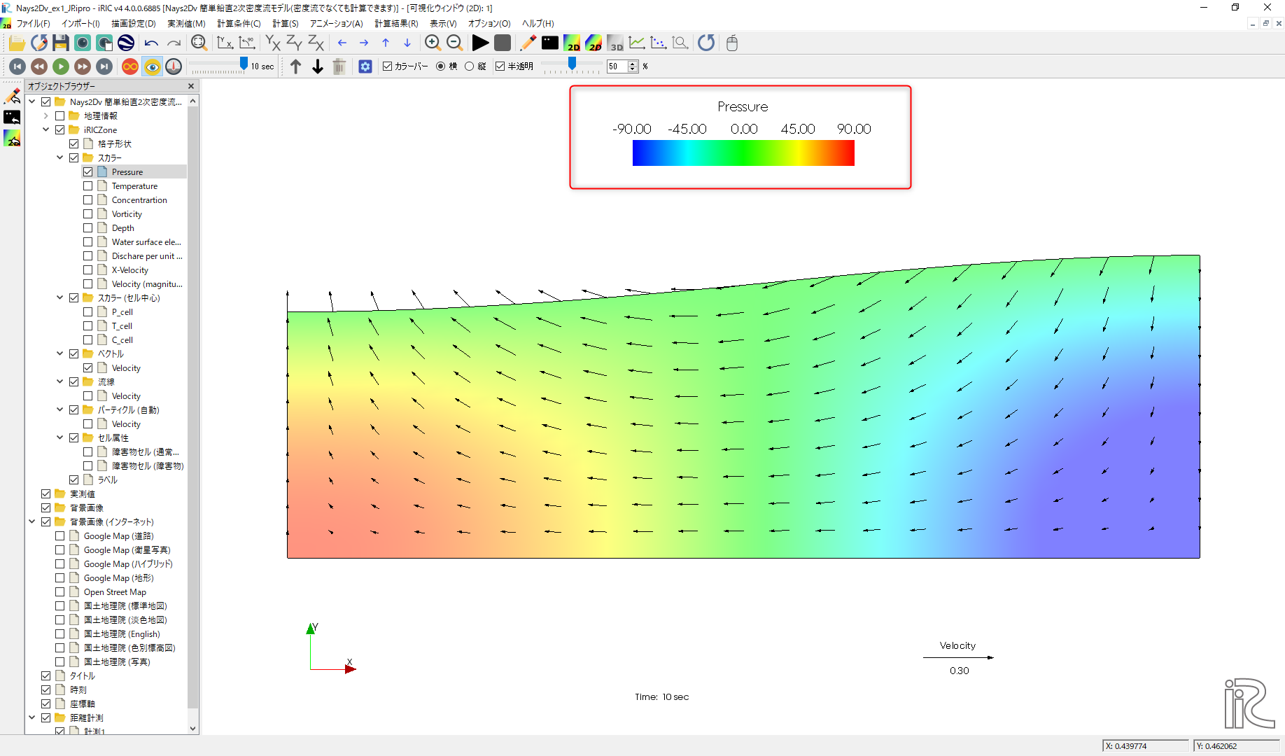
../_images/kekka_9.png — 図 25 : 圧力コンター設定終了

以下、ベクトルと同様にアニメーション表示も出来る。図 26

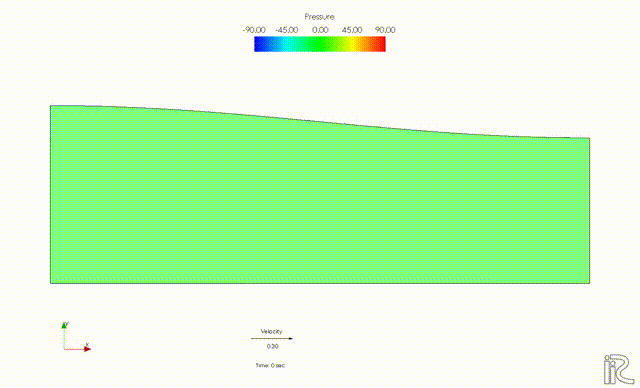
../_images/ex1.gif — 図 26 : 圧力コンターと流速ベクトルのアニメーション