[Example 2] Flow in a 360 degree circle channel
Create Computational Grid
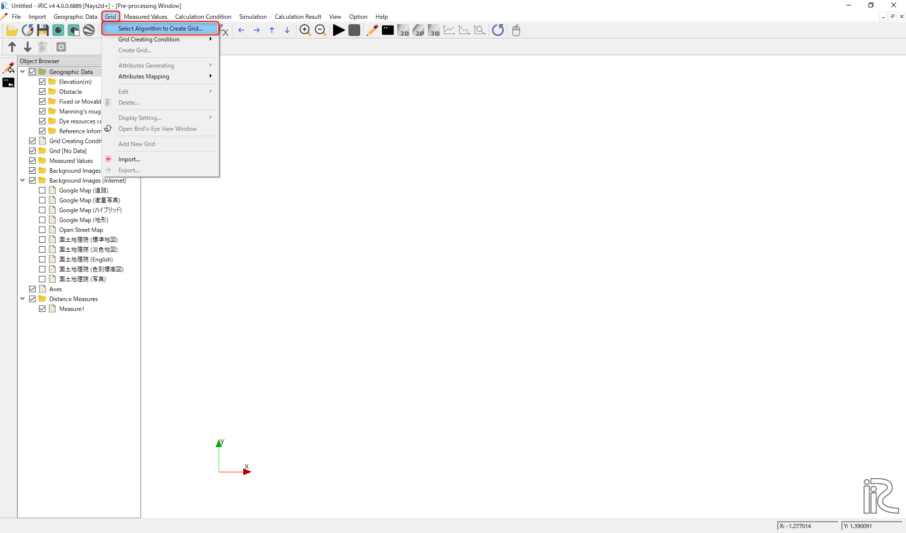
Figure 34 : Select Algorithm
From the main menu, select [Grid], [Select Algorithm to Create Grid] ( Figure 34 ) Then the [Select Grid Creating Algorithm] window, Figure 35 appears. Select [2d arc generator] and click [OK]
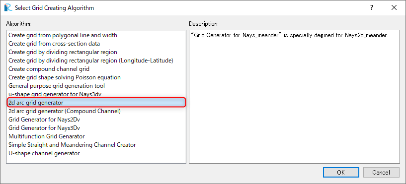
Figure 35 :Select Grid Creating Algorithm
Set values as shown in Figure 36 , and click [OK]. Click [Yes] when you asked “Do you want to map data?” as Figure 37 . Then the computational grid appears.
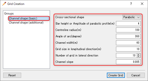
Figure 36 : Grid Creation: Channel Shape (Basic)
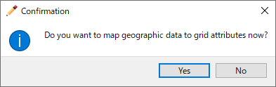
Figure 37 : Mapping
Bed configuration can be confirmed by putting checking marks at, [Grid], [Node attributes] and [Elevation (m)]. ( Figure 38 )
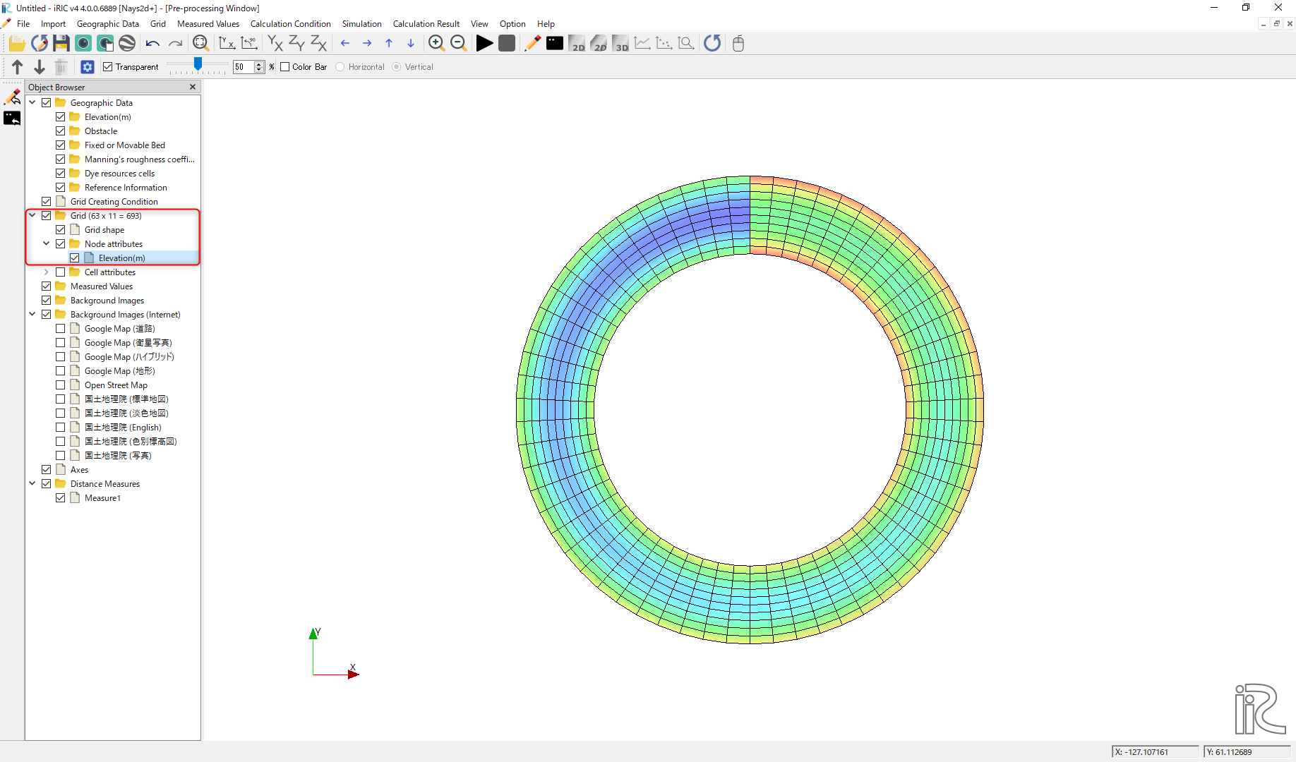
Figure 38 : Grid Creation Completed
Computational Condition
From the menu bar, select [Calculation Condition], [Settins] and [Calculation Condition] window, Figure 39 appears.
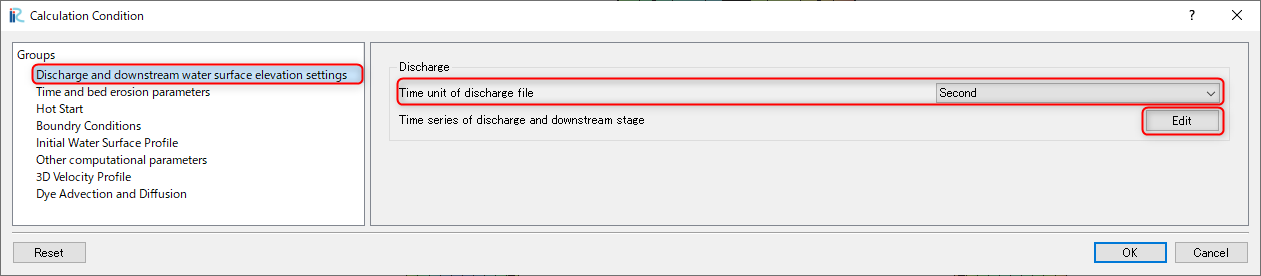
Figure 39 : Calculation Condition: Groups
In Figure 39 , select [Discharge and downstream water surface elevation] and click [Edit].
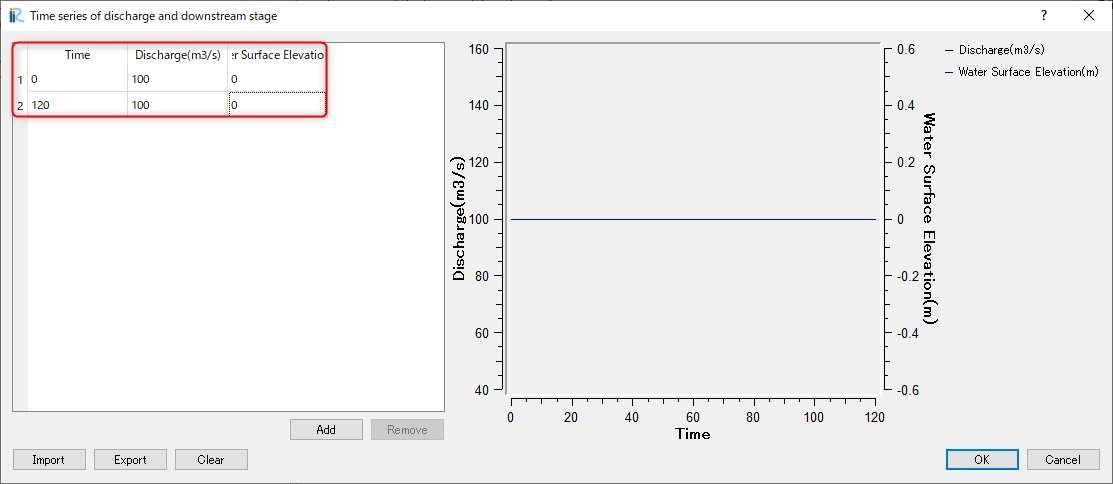
Figure 40 : Input discharge hydro graph
Input dischege hydrograph as shown in Figure 40 and click [OK].
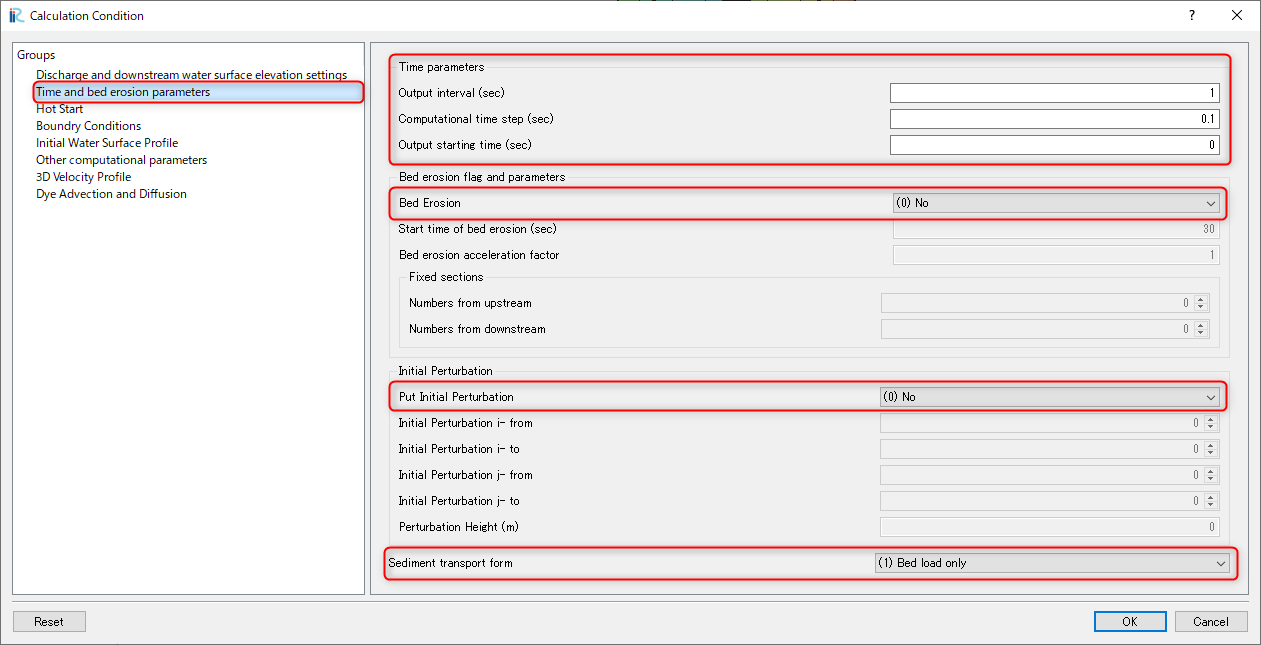
Figure 41 : Time and bed erosion parameters
Select [Time and bed erosion parameters] and set values as Figure 41 .
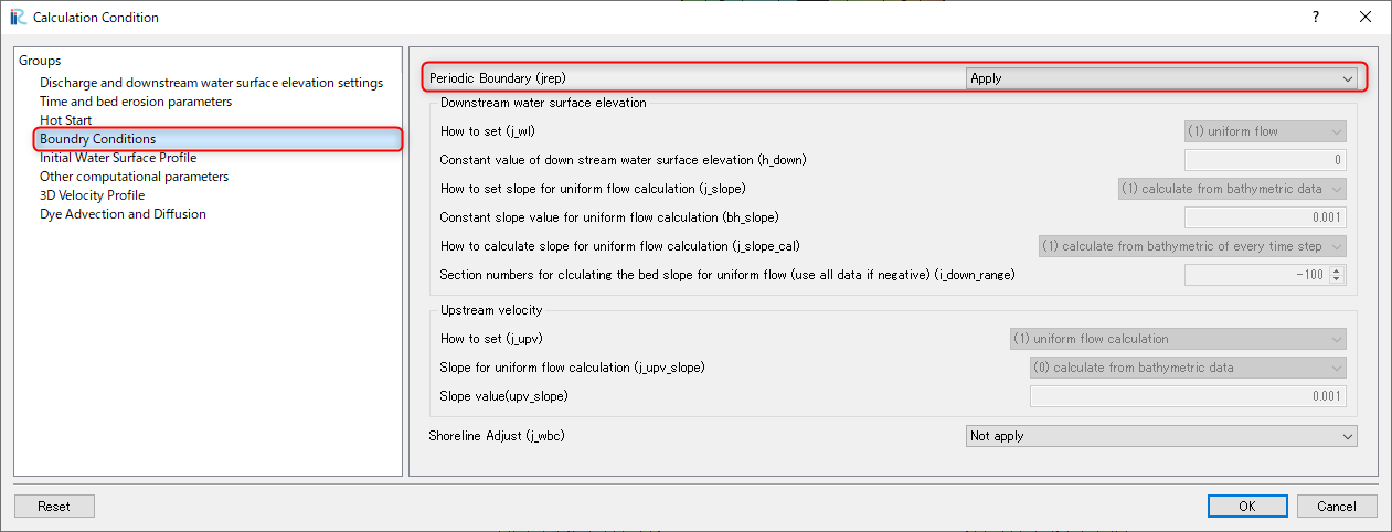
Figure 42 : Boundary Condition
Set [Boundary Condition] as Figure 42
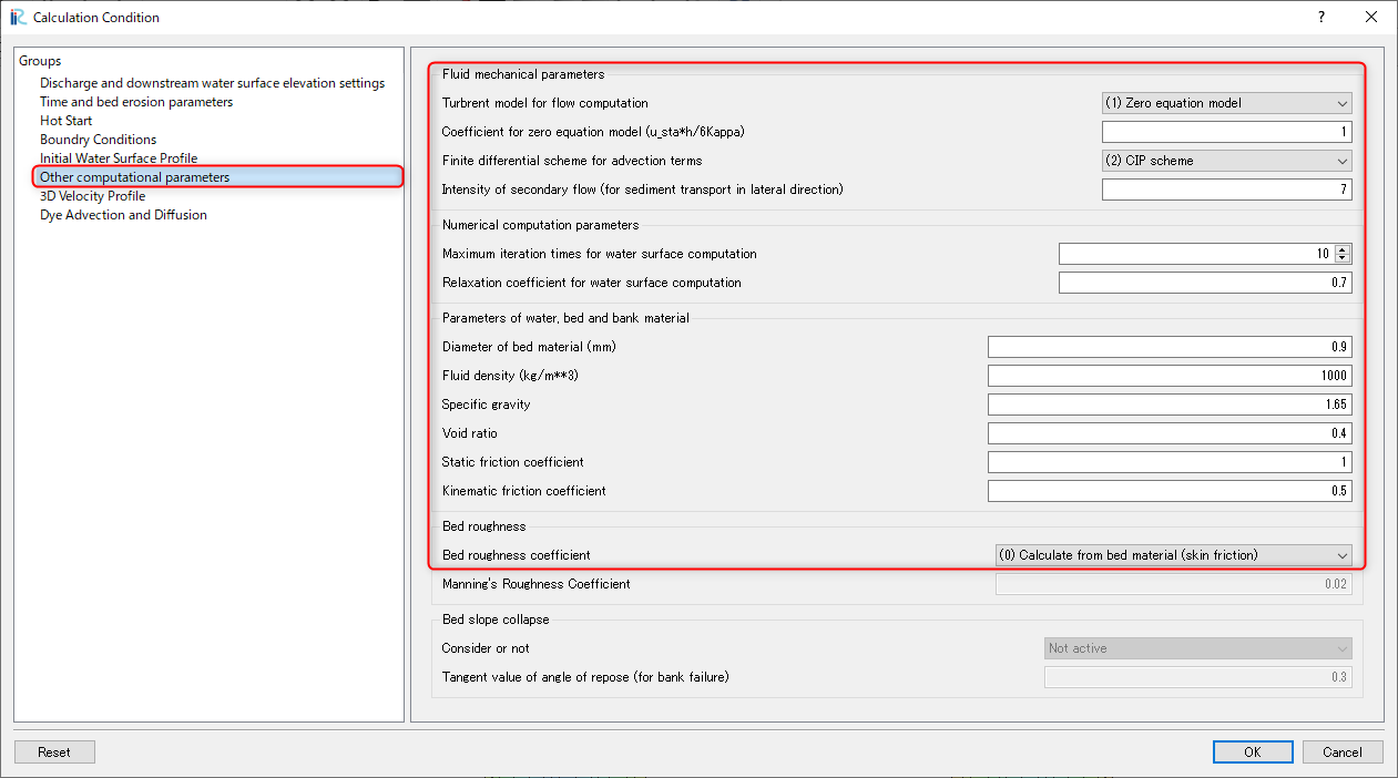
Figure 43 : Other computational parameters
Set [Other computational parameters] as Figure 43
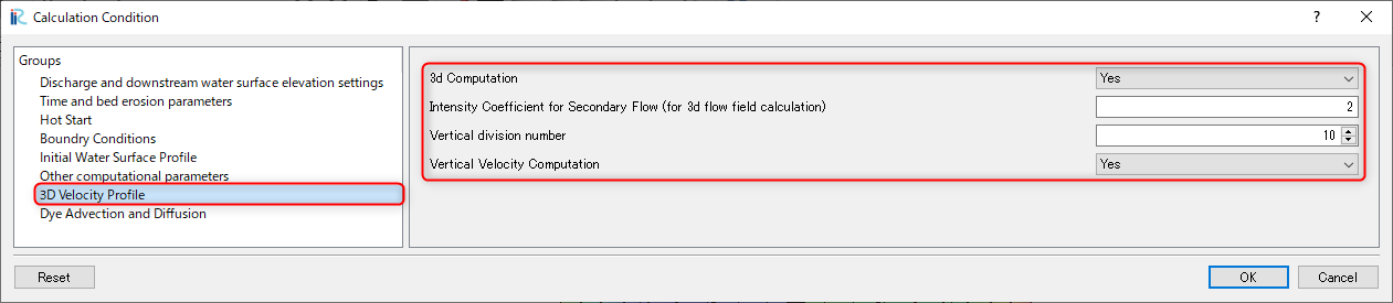
Figure 44 : 3D Velocity Profile
Set [3D Velocity Profile] as Figure 44, and click [OK]
Launch Computation
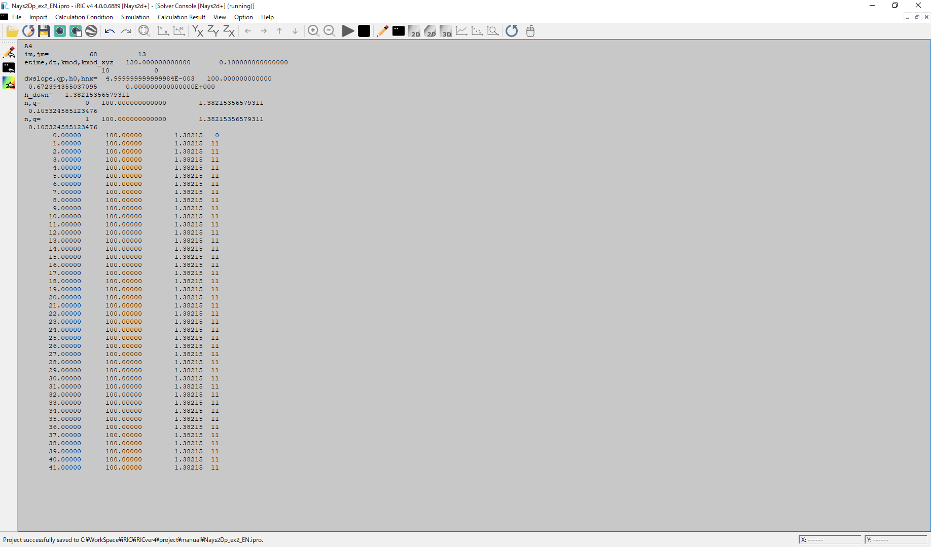
Figure 45 :Launch Computational
By selectng [Simulation] and [Run], a window as Figure 45 appears, and the simulations starts.
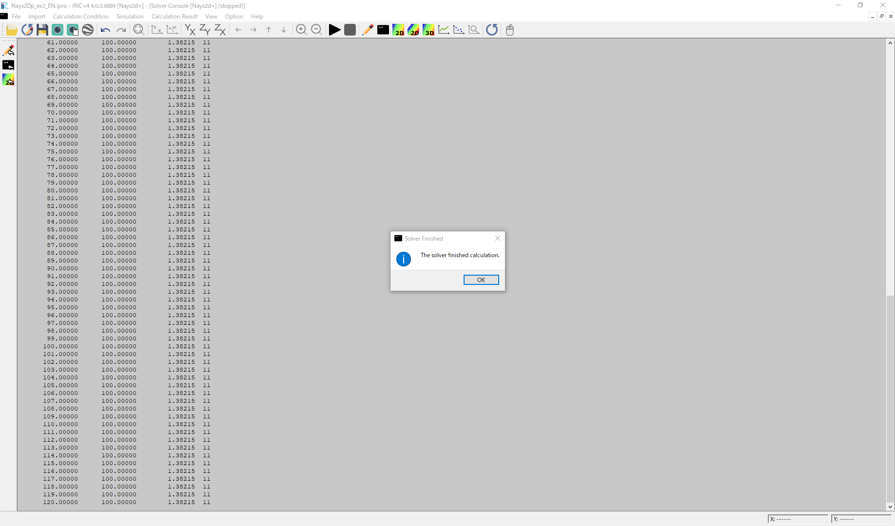
Figure 46 :Simulation Fished
When the simulation finish, Figure 46 appears. Then click [OK].
Display Computational Results
After the companion finished, form the main menu, by selecting [Calculation Results] and [Open new 2D Post-Processing Window], a new Window appears as Figure 47 .
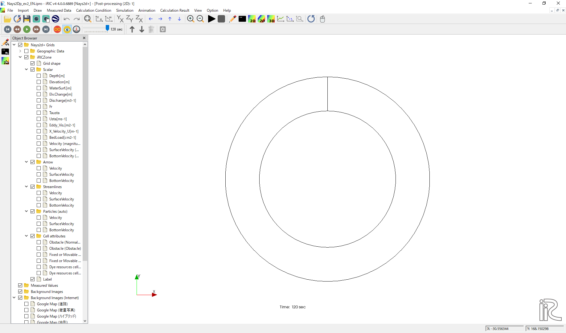
Figure 47 :2D Post-Processing Window
Depth
In the object browser, put the check marks in “Scalar (node)” and “Depth[m]”, right-click and select “Properties”. The “Scalar Setting” window Figure 48 appears.
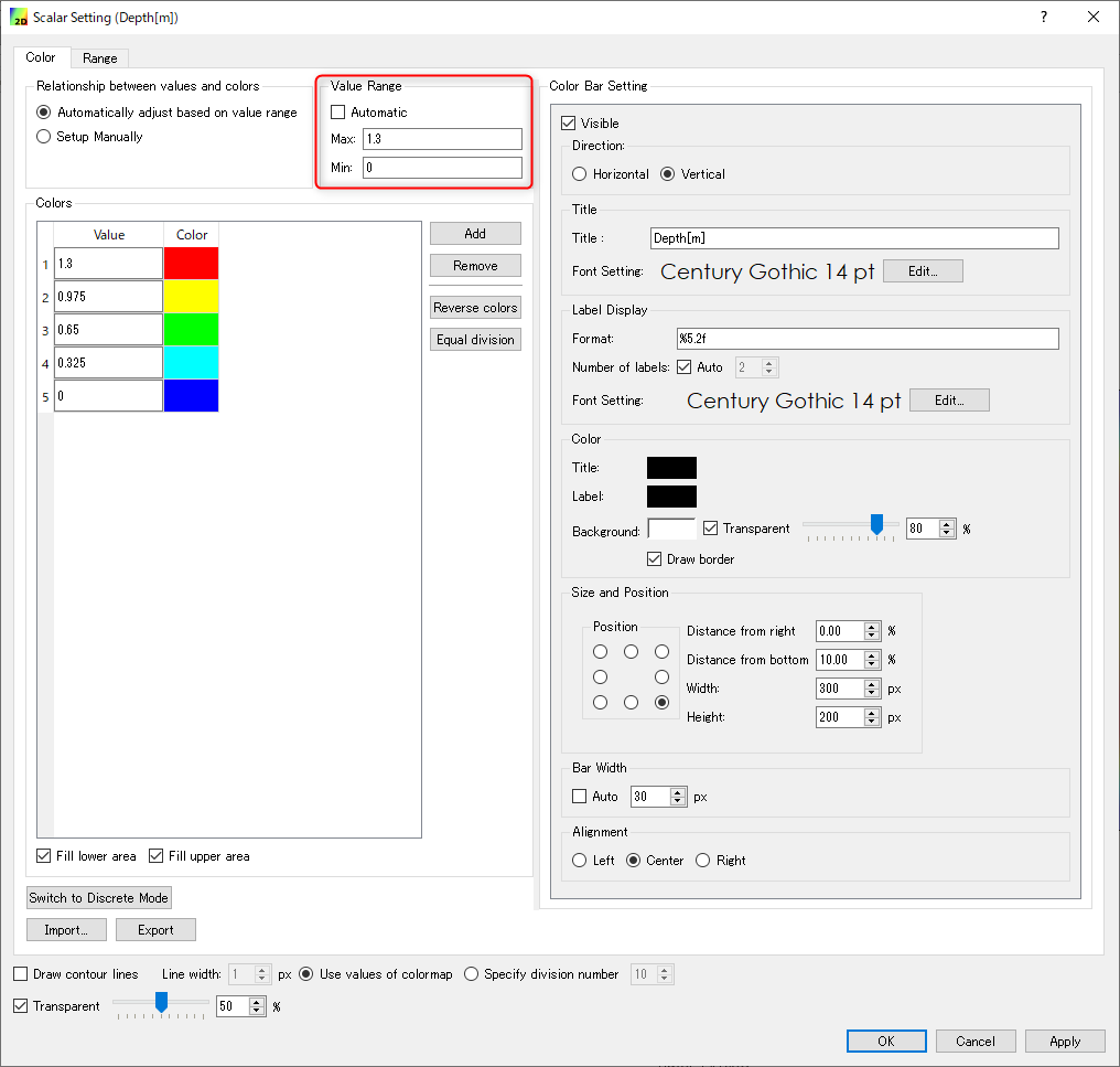
Figure 48 :Scalar Setting
Set the values as shown in Figure 48, and click [OK], then Figure 49 appears.
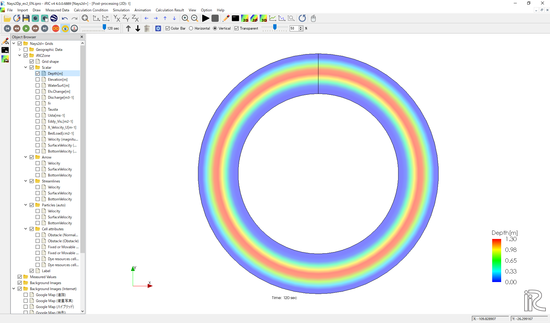
Figure 49 : Depth Plot
Velocity vectors
In the object browser, put the check marks in “Arrow” and “Velocity”, right-click and select “Properties”. The “Arrow Setting” window Figure 50 appears. Set the values as Figure 50, and click [OK].
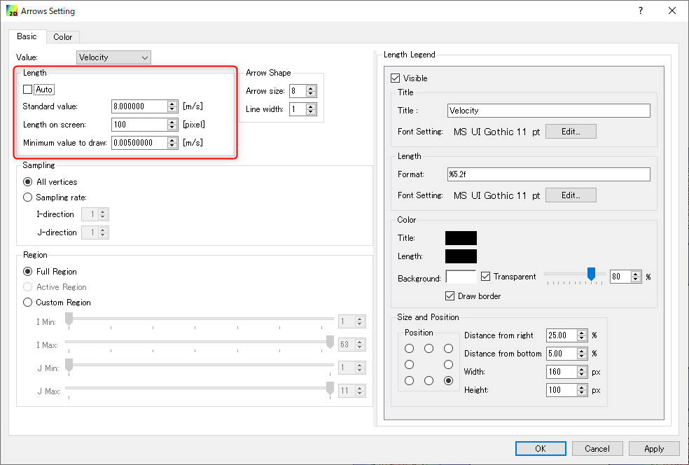
Figure 50 :Arrow Setting
Figure 51 shows the depth-averaged velocity vectors.
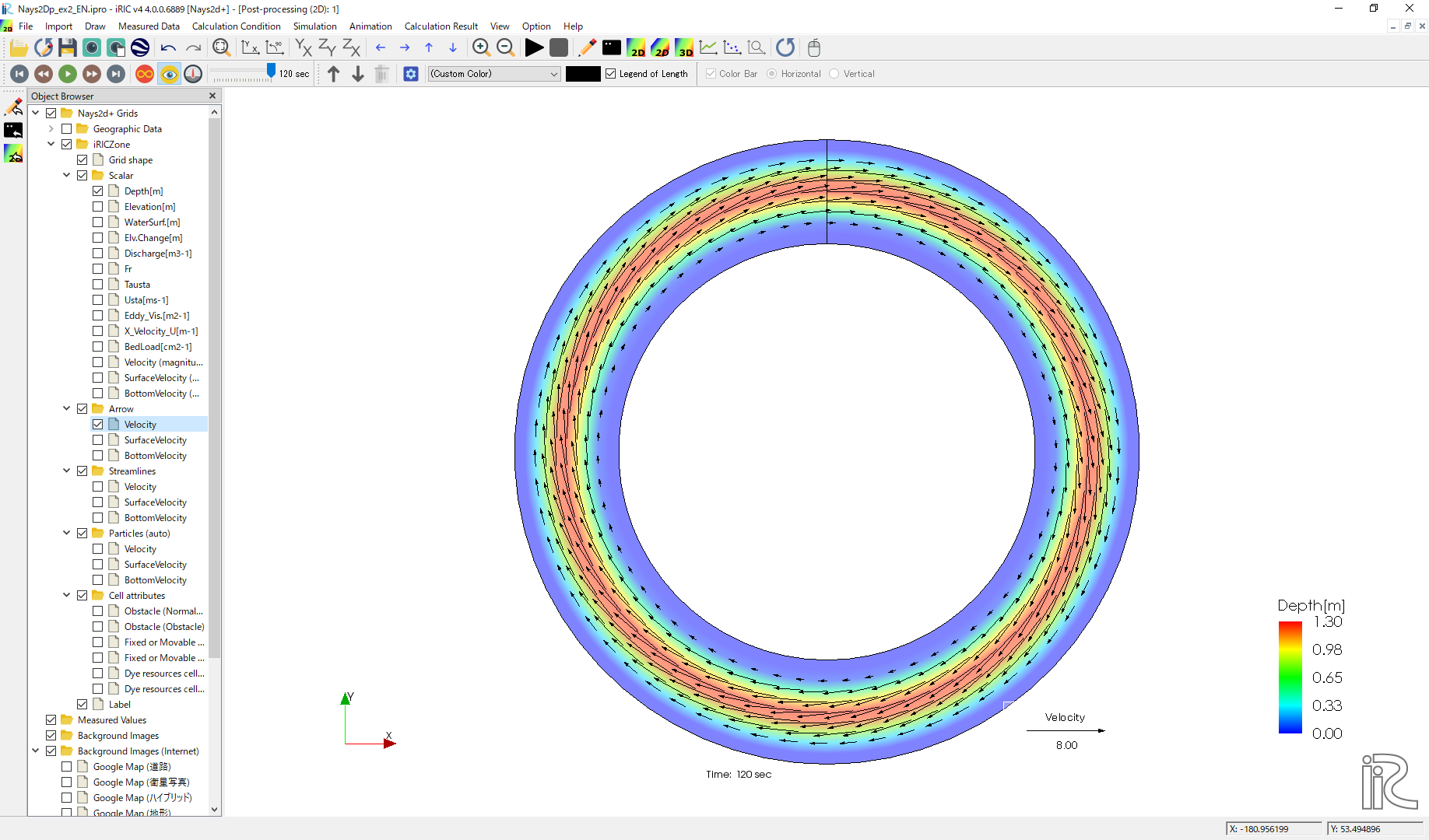
Figure 51 :Depth Averaged Velocity Vectors
In Figure 51, you can select “Surface Velocity” and “Bottom Velocity” by chekking each box in “Arrow” group.
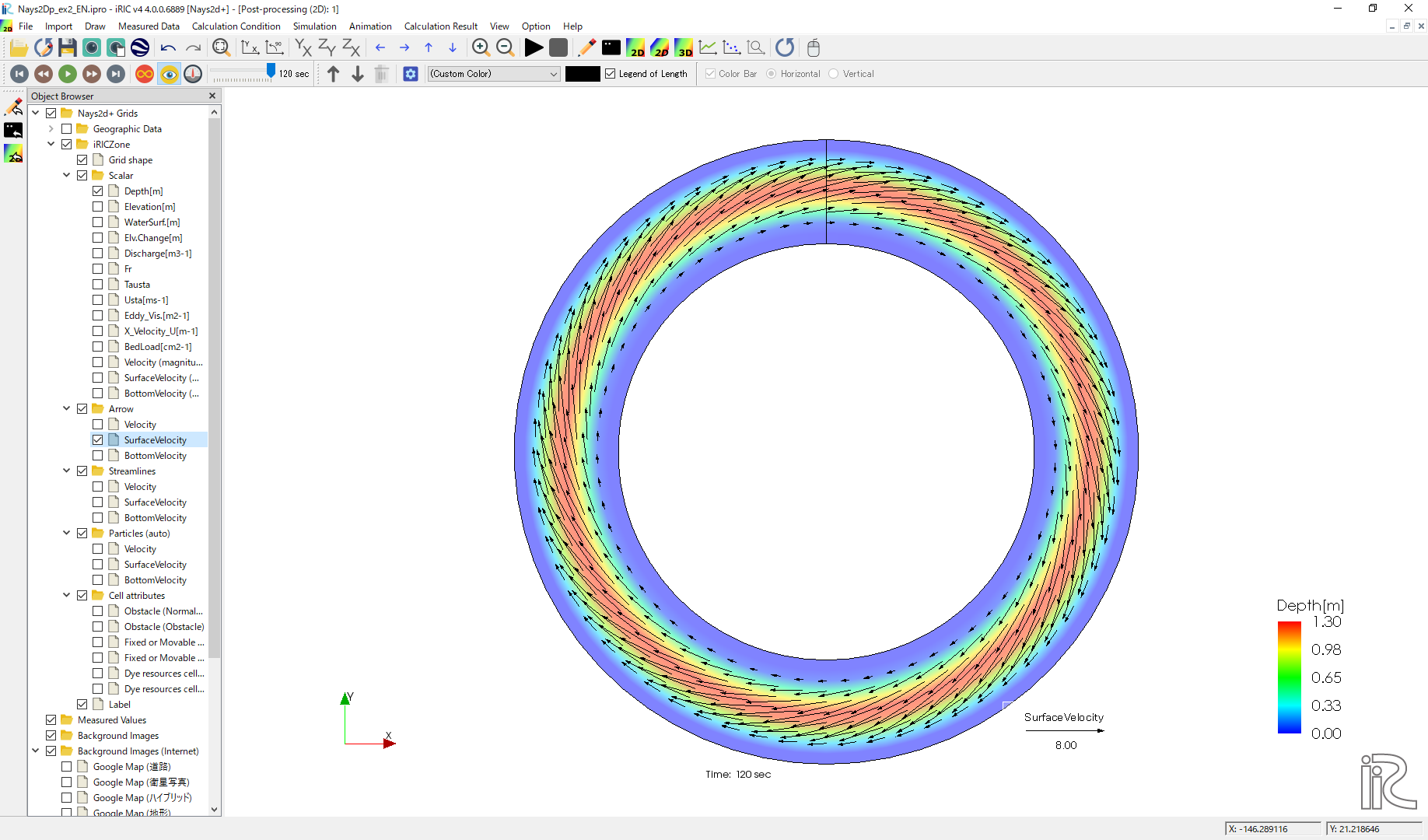
Figure 52 : Surface Velocity Vectors
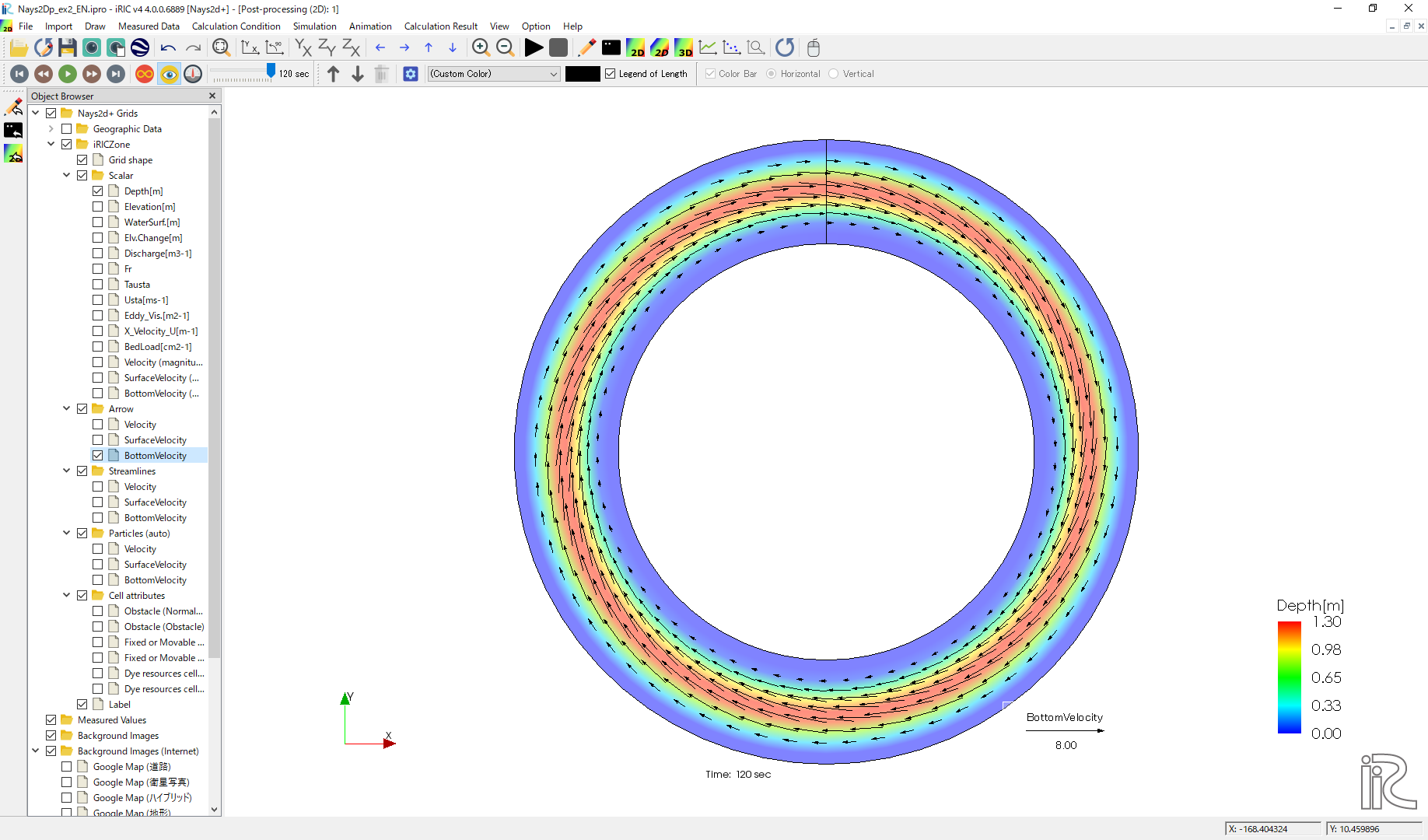
Figure 53 : Bottom Velocity Vectors
Stream Lines
Uncheck the box by “Arrow” in the Object Browser and check a box by “Streamline”. By checking “Velocity”, the streamlines following the depth averaged flow velocity” Figure 54 will be displayed. By checking “Surface Velocity”, the streamline following the surface velocity” Figure 55 will be displayed. By checking “Bottom Velocity”, the streamline following the bottom velocity ne: numref:02_kekka_11 will be displayed.
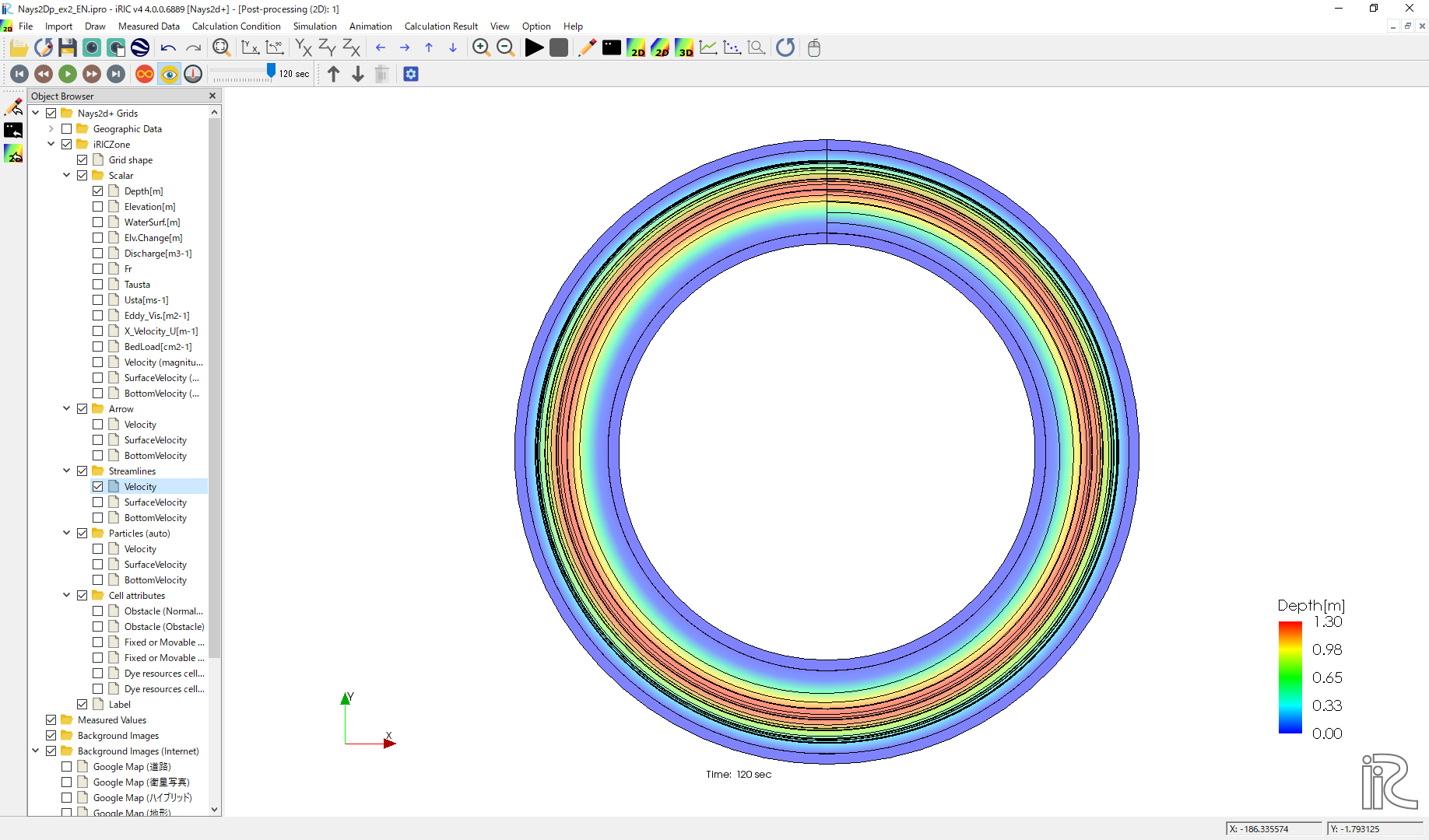
Figure 54 :Streamlines by depth averaged velocity
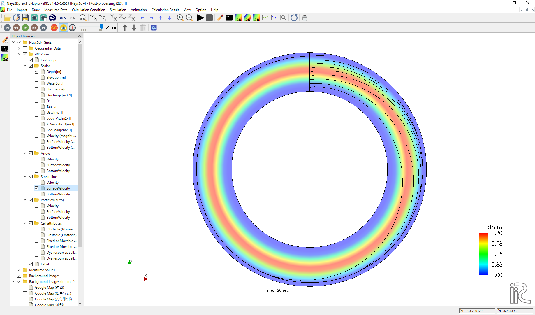
Figure 55 :Streamlines by surface velocity
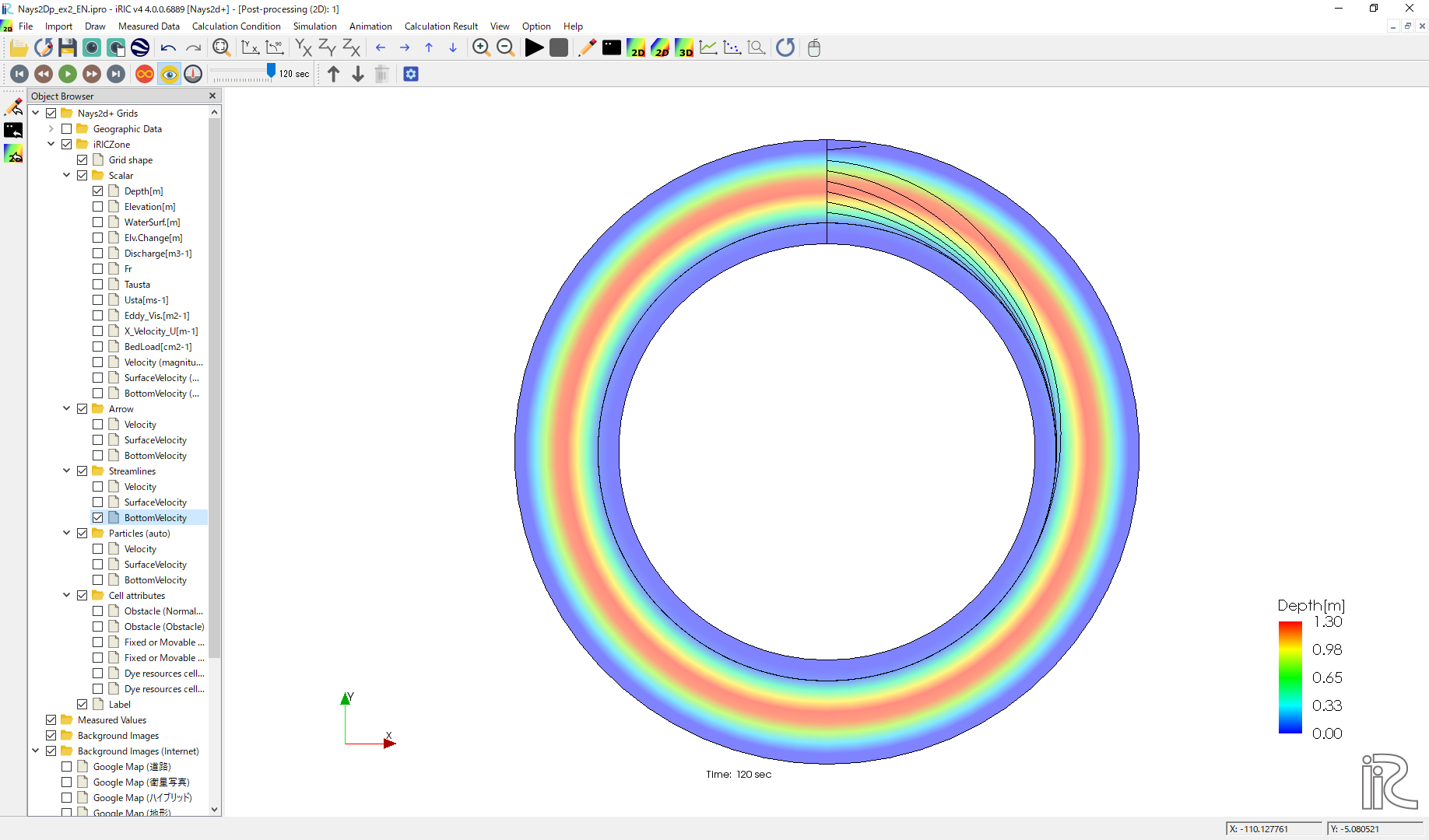
Figure 56 :Streamlines by bottom velocities
The effect of the secondary flow is clearly shown.