[Example 5] Flow in a Real River (Compound Cross section)
Select Solver
In the [Select Solver] window, Figure 130 , select [Nays2d+] and click [OK].
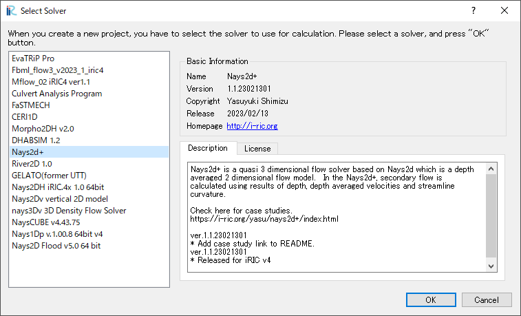
Figure 130 : Select Solver
Importing River Survey Data
In the window, Figure 131, select [Import], [Geographic Data], [Elevation(m)]
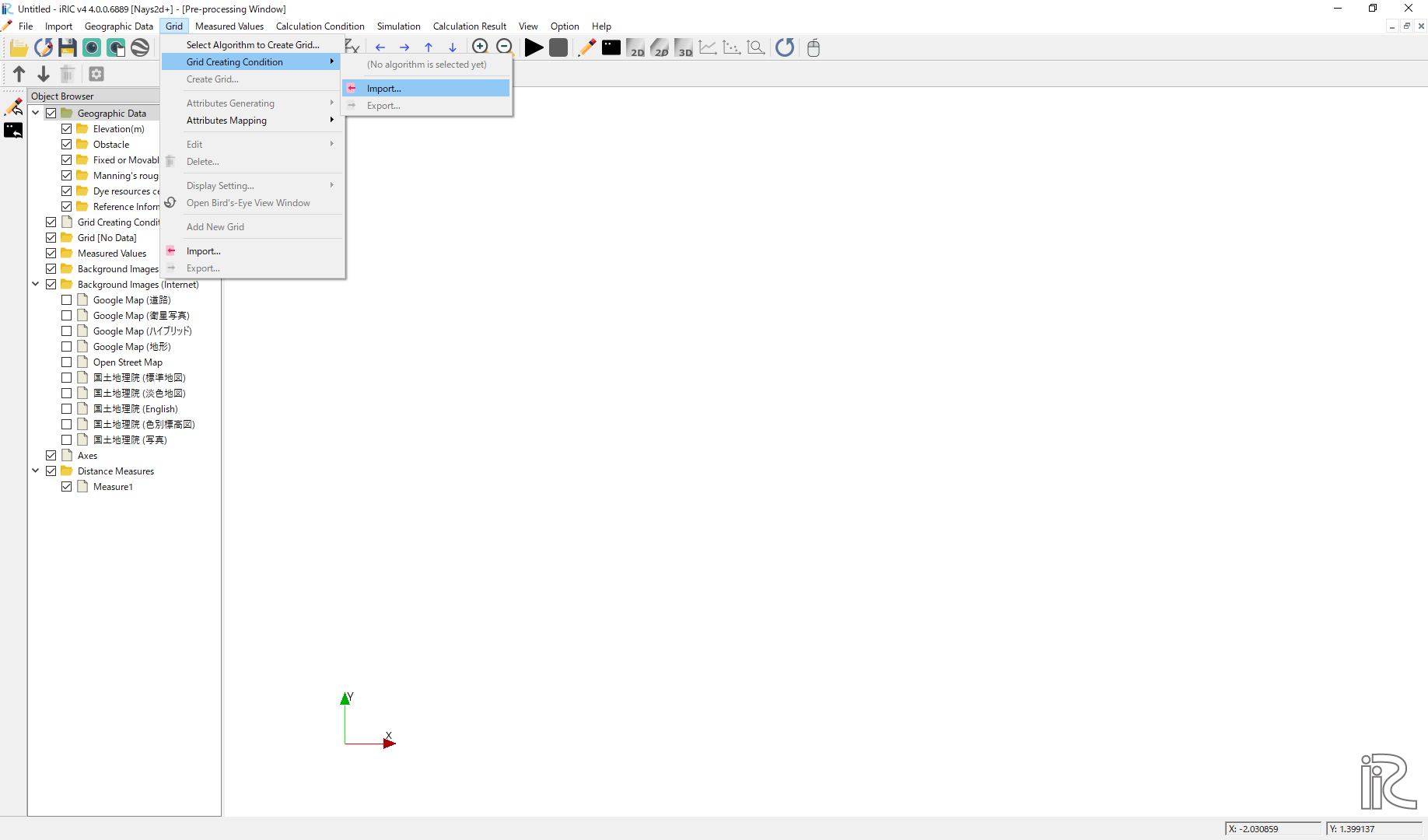
Figure 131 : Import river geographic data
Chose [compound.riv] in the window, Figure 132 and open. The cross sectional survey data “compound.riv” can be downloaded from, https://i-ric.org/yasu/fw/rivfiles/compound.riv
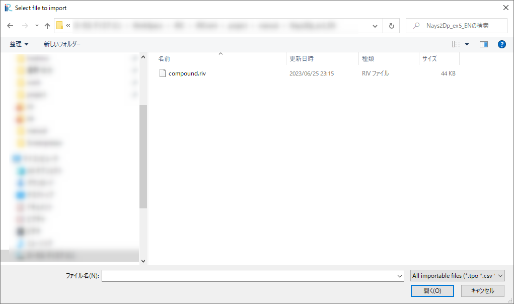
Figure 132 : Select File
A message window may appear telling “Problems Fund i Data” as Figure 133 ,but just click [OK]
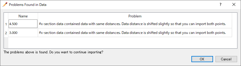
Figure 133 : Problem Fund
Select [Middle point of left and right bank] in the [River Survey Data Import Setting] window as Figure 134 , and click [OK]
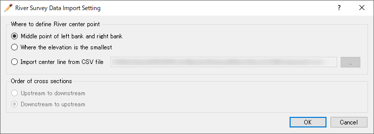
Figure 134 : River Survay Data Import Setting
Figure 135 riv file import complete.
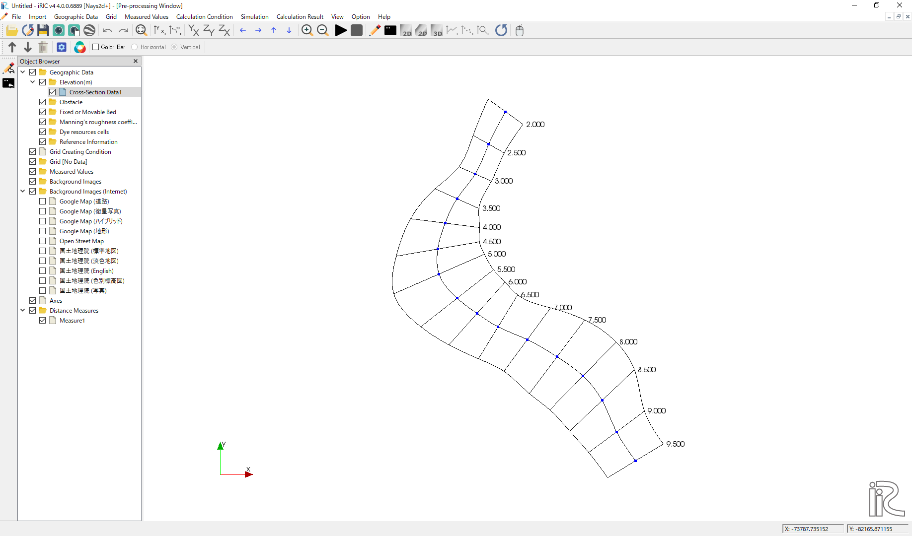
Figure 135 : Import Complete
Moving centerline
As shown in Figure 136 , move the centerline of the channel close to approximate center of the low water channel.
Figure 136 : Moving Centerline
Grid Generation Conditions
From the main menu, select [Grid] and [Select Algorithm to Create Grid] as, Figure 137
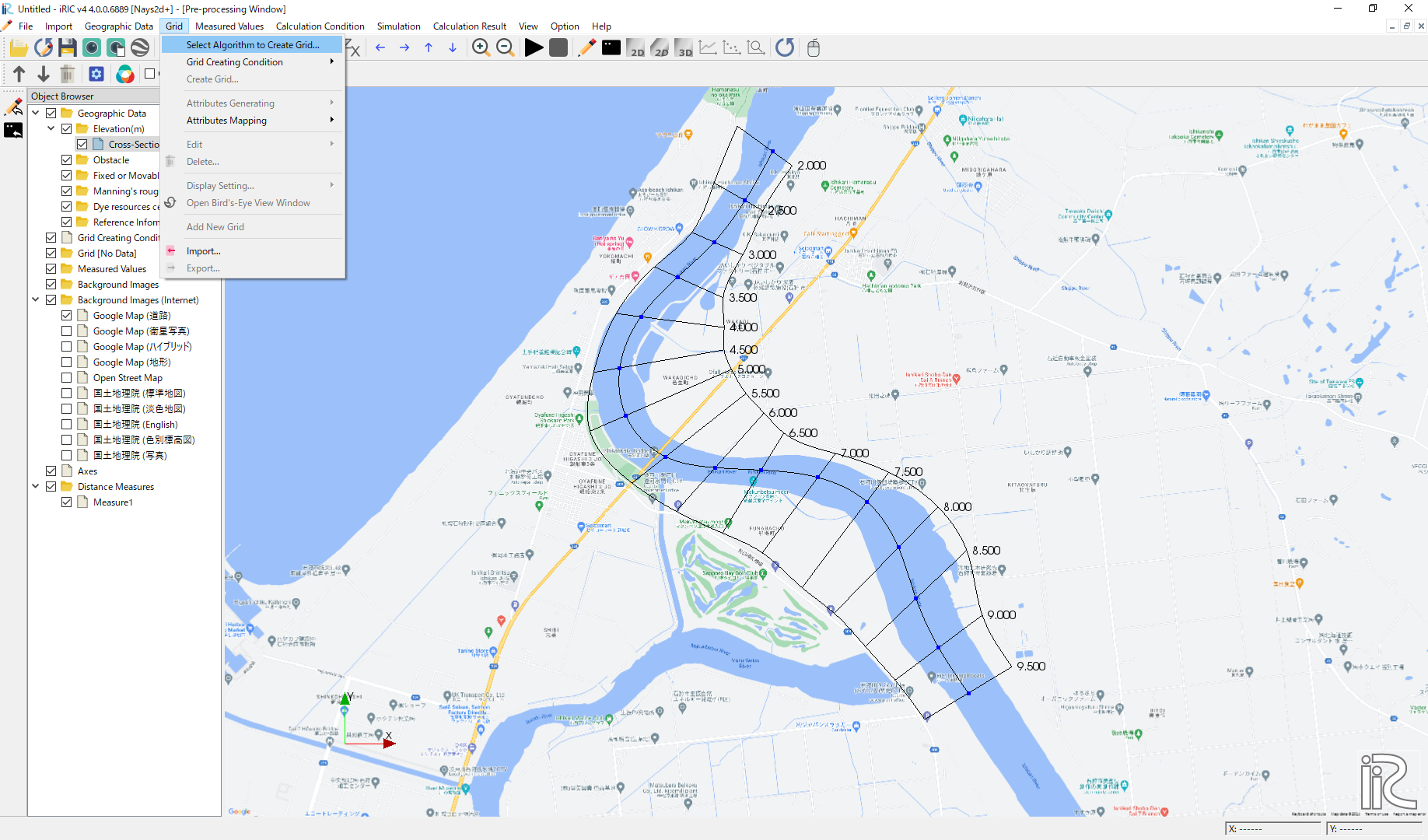
Figure 137 : Select Algorithm to Create Grid
Select [Create grid from river survey data] from the window, Figure 138 , and click [OK].
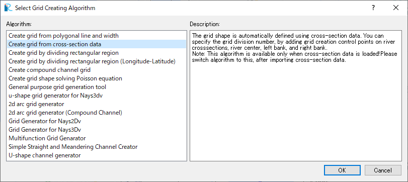
Figure 138 :Create grid from river survey data
As shown in Figure 139 , a channel with cross sections with both ends’ blue circles are displayed.
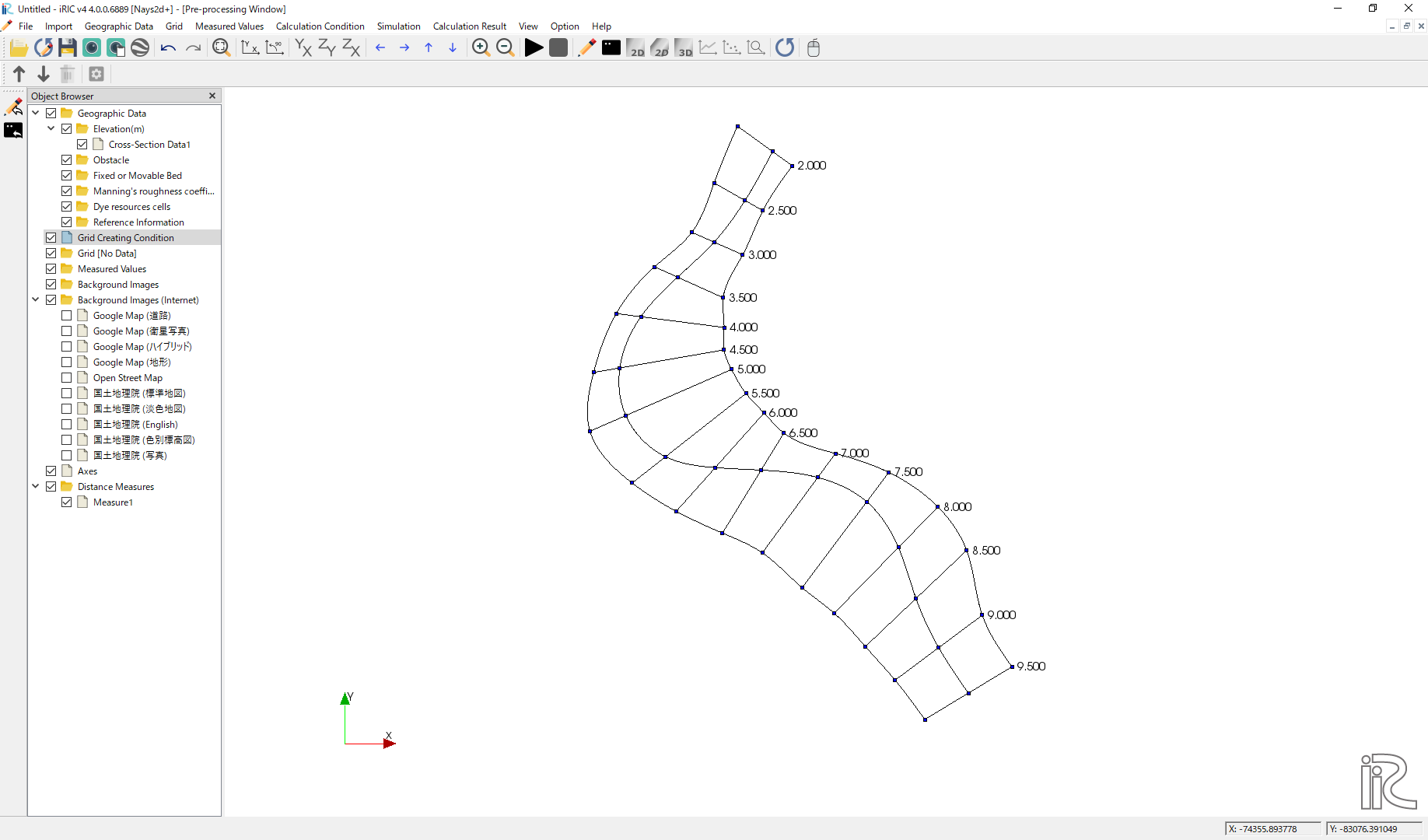
Figure 139 : Setting Grid Create Condition Complete
Grid Generation
Select any side of one of the cross section line, right click, and chose [Add Division Points].
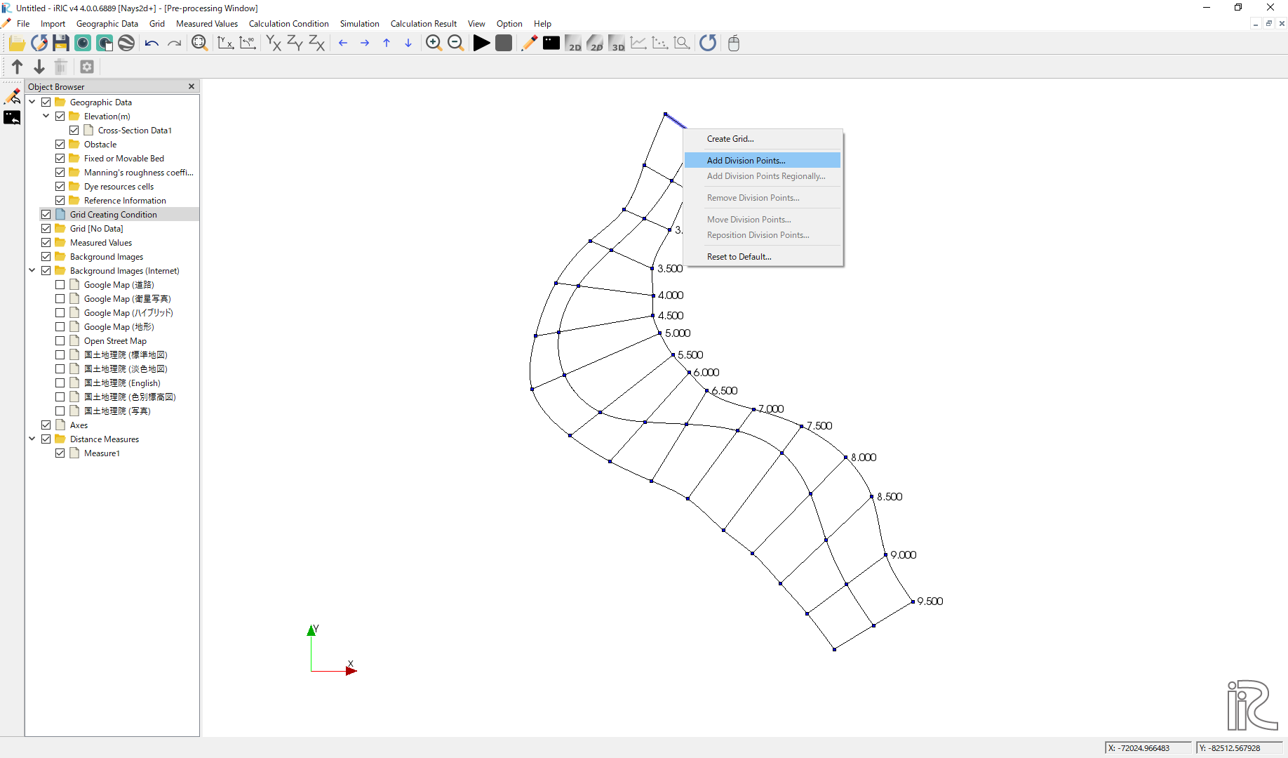
Figure 140 :Add Division Points(1)
Set [Division Number], set [8] in this example, and click [OK] (Figure 141 )
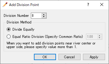
Figure 141 :Add Division Points(2)
Select one of the opposite side of the cross sectional line we selected in Figure 140 , right click, and chose [Add Division Points] (Figure 142 )
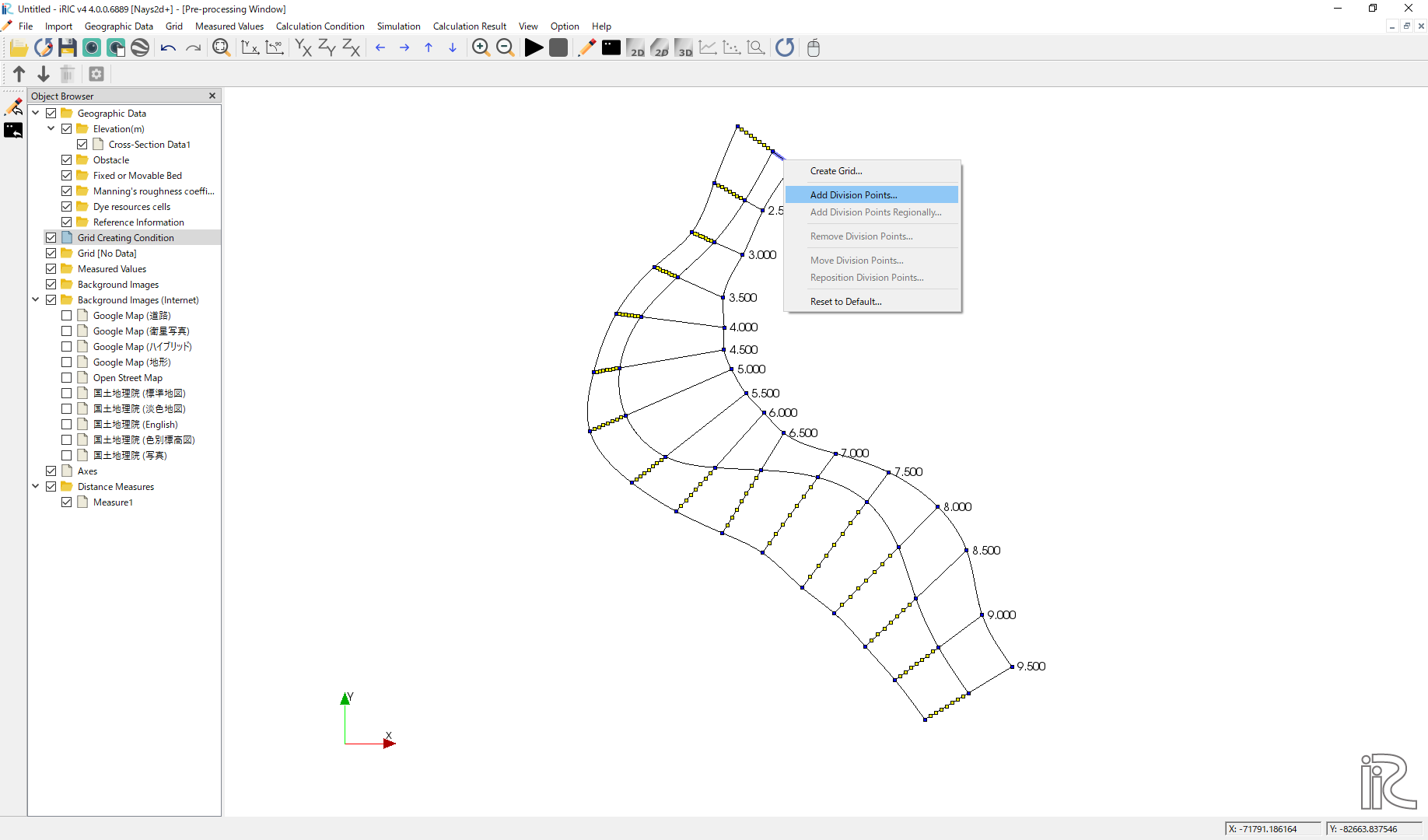
Figure 142 :Add Division Points(3)
Set [Division Number], set [8] as a same number we set in Figure 141 for the symmetry.

Figure 143 :Add Division Points(4)
Along the channel direction, division points are set all at once. Select [Grid], [Add Division Points Regionally] from the menu bar. ( Figure 144 )
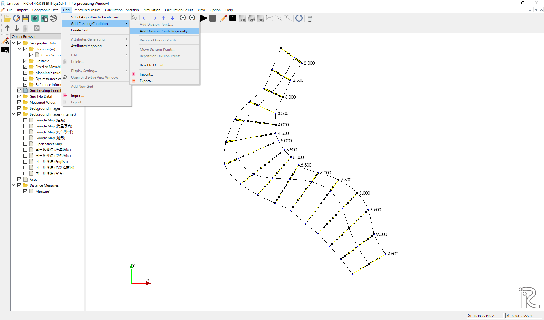
Figure 144 :Add Division Points Regionally(1)
Chose [Specify target distance division points]. set distance [50] in this example, and click [OK].( Figure 145 )
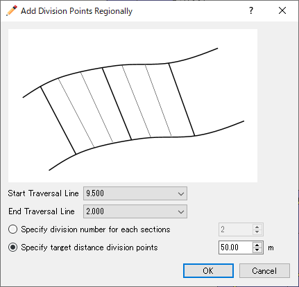
Figure 145 :Add Division Points Regionally(2)
When the setup for division points are completed, a plane map with yellow circle points appears as Figure 146
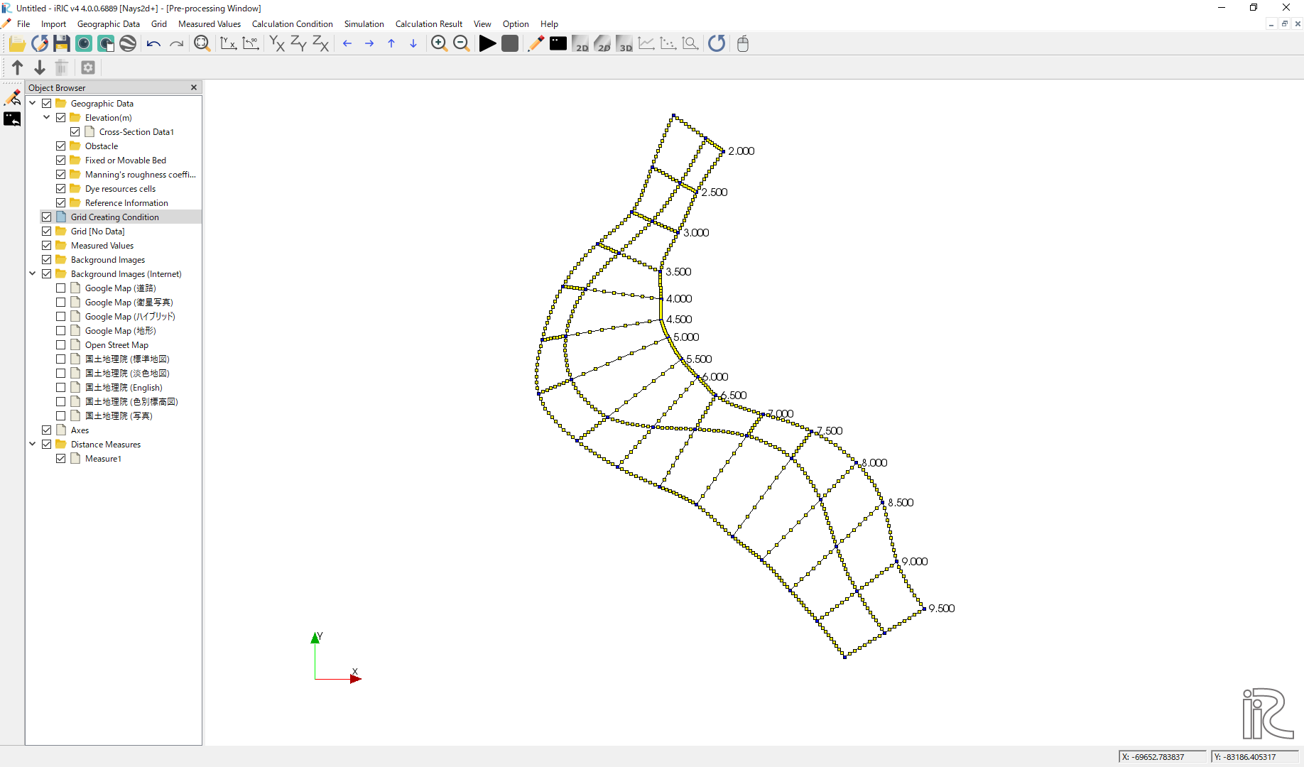
Figure 146 :Set division points complete
Select [Grid], [Grid Create] from the menu bar.( Figure 147 )
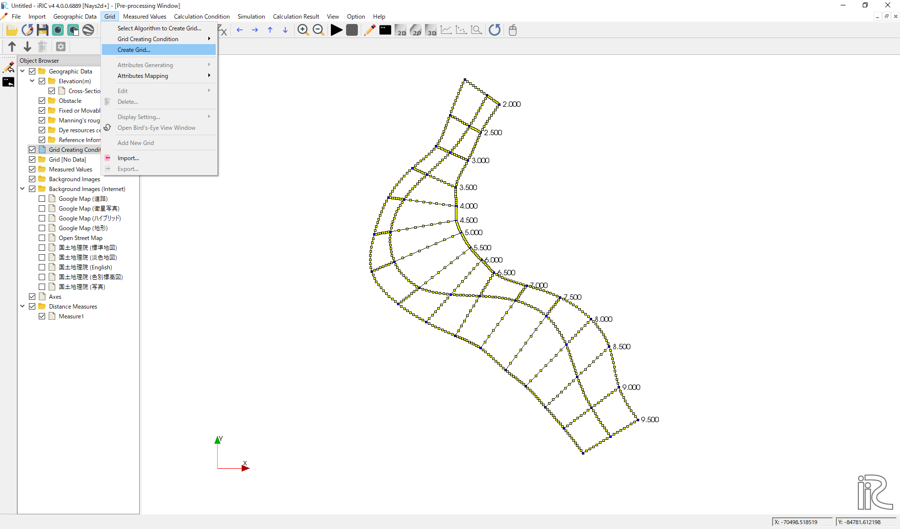
Figure 147 :Grid Create(1)
Confirm the grid generation range painted with blue, and click [OK].
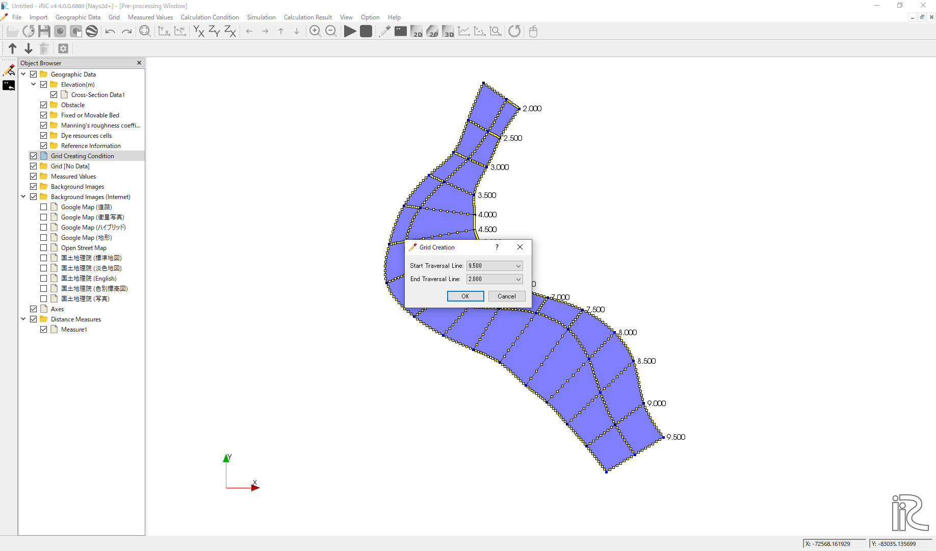
Figure 148 :Grid Create(2)
Answer [Yes] when you asked [Do you want to map?] as Figure 149
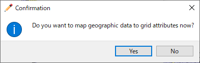
Figure 149 :Mapping?
Completed grid is shown as Figure 150
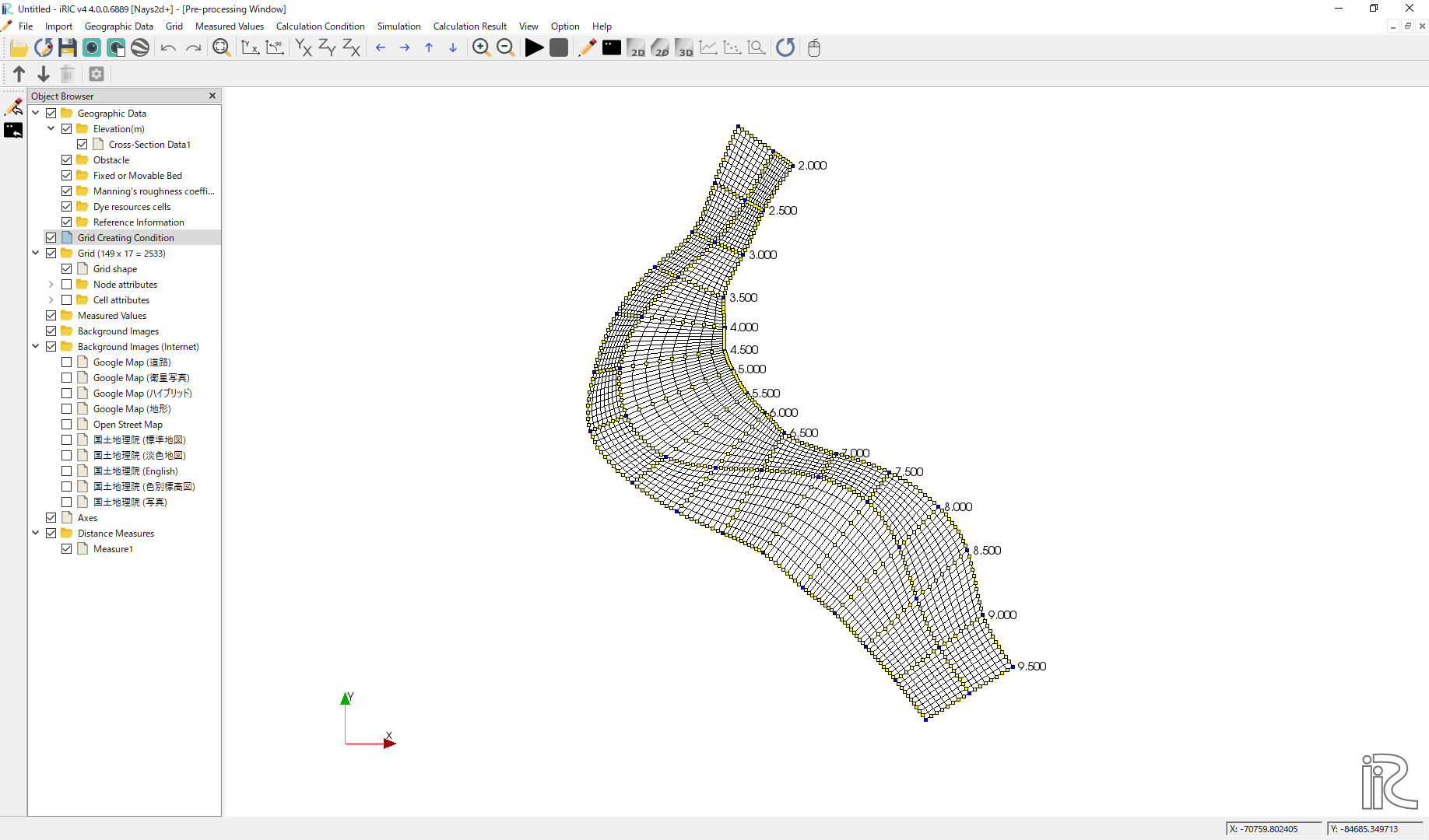
Figure 150 :Grid Generation Complete
Bed configuration and channel shape can be confirmed by putting checking marks at, [Grid], [Node attributes] and [Elevation (m)]. ( Figure 151 )
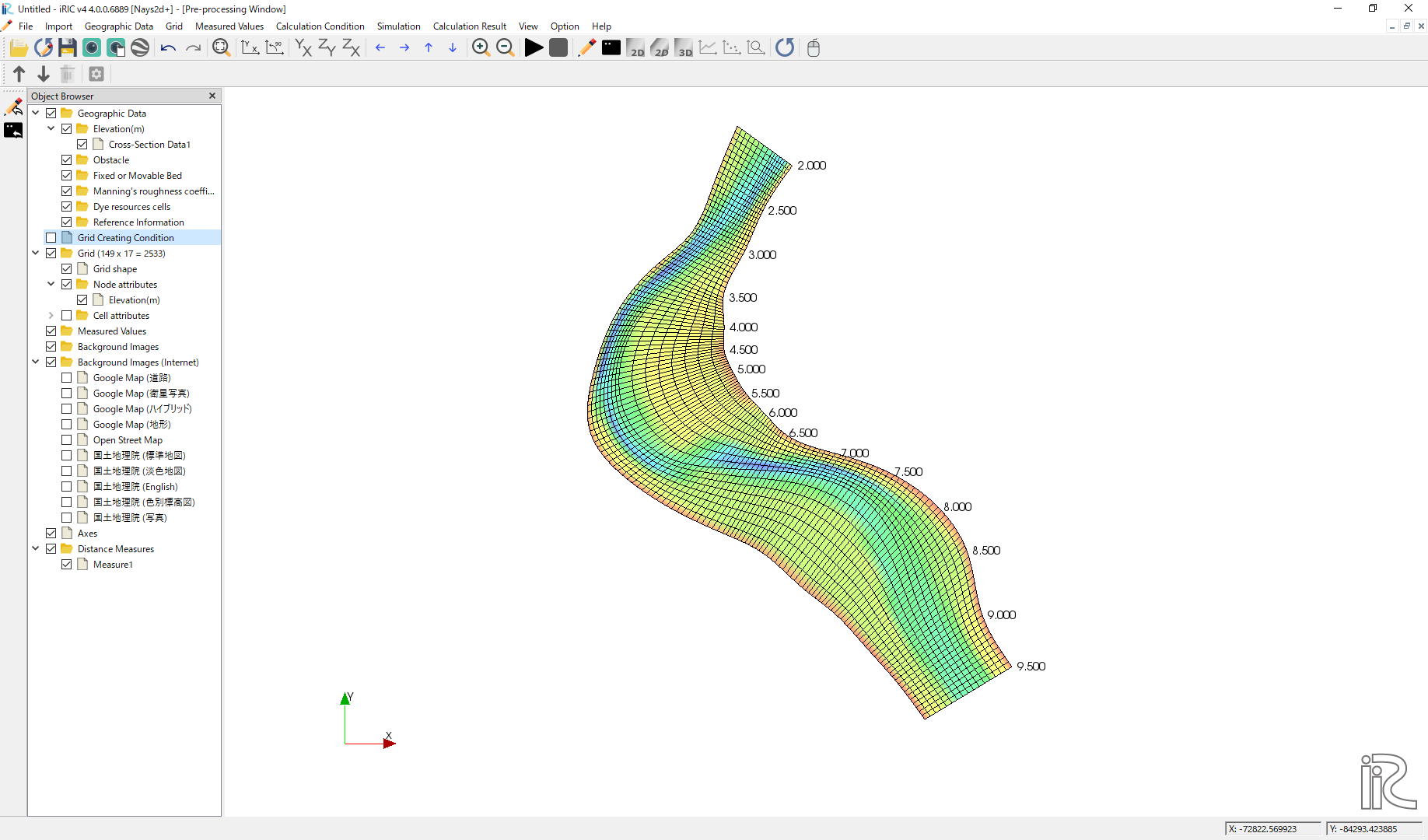
Figure 151 :Confirmation of the Mapping Result
Computational Condition
Select [Calculation Condition] and [Setting] from the min menu as Figure 152 .
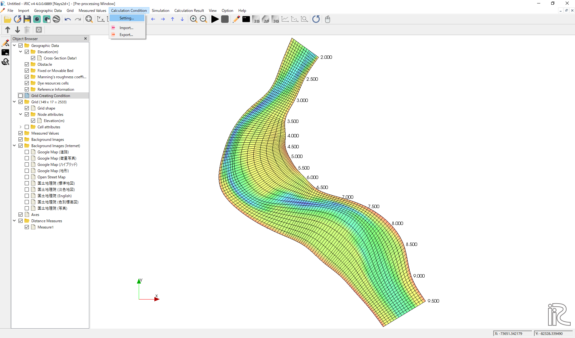
Figure 152 :Setting Computational Condition
Set [Time unit of discharge] as [Hour] and click [Edit], ( Figure 153 )
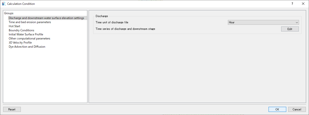
Figure 153 :Discharge Condition
Set discharge hydrography as Figure 154, constant for 3 hours with 2,000 qms, and click [OK].
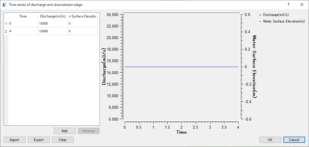
Figure 154 :Input Discharge(2)
Set [Time and bed erosion condition] as Figure 155 .
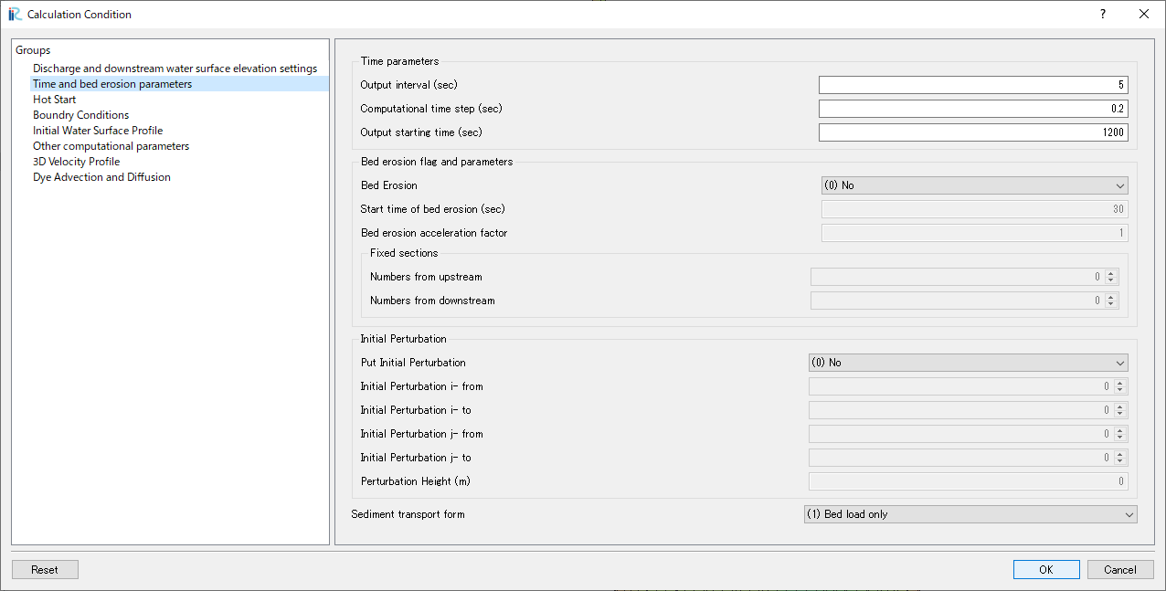
Figure 155 :Time and bed erosion condition
Set [Boundary Conditions] as Figure 156 .
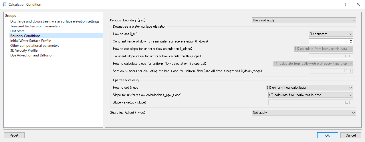
Figure 156 :Boundary Conditions
Set [Initial Water Surface Profile] as Figure 157 .
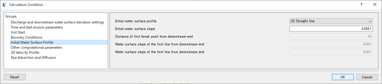
Figure 157 :Initial Water Surface Profile
Set [Other computational parameters] as Figure 158 .
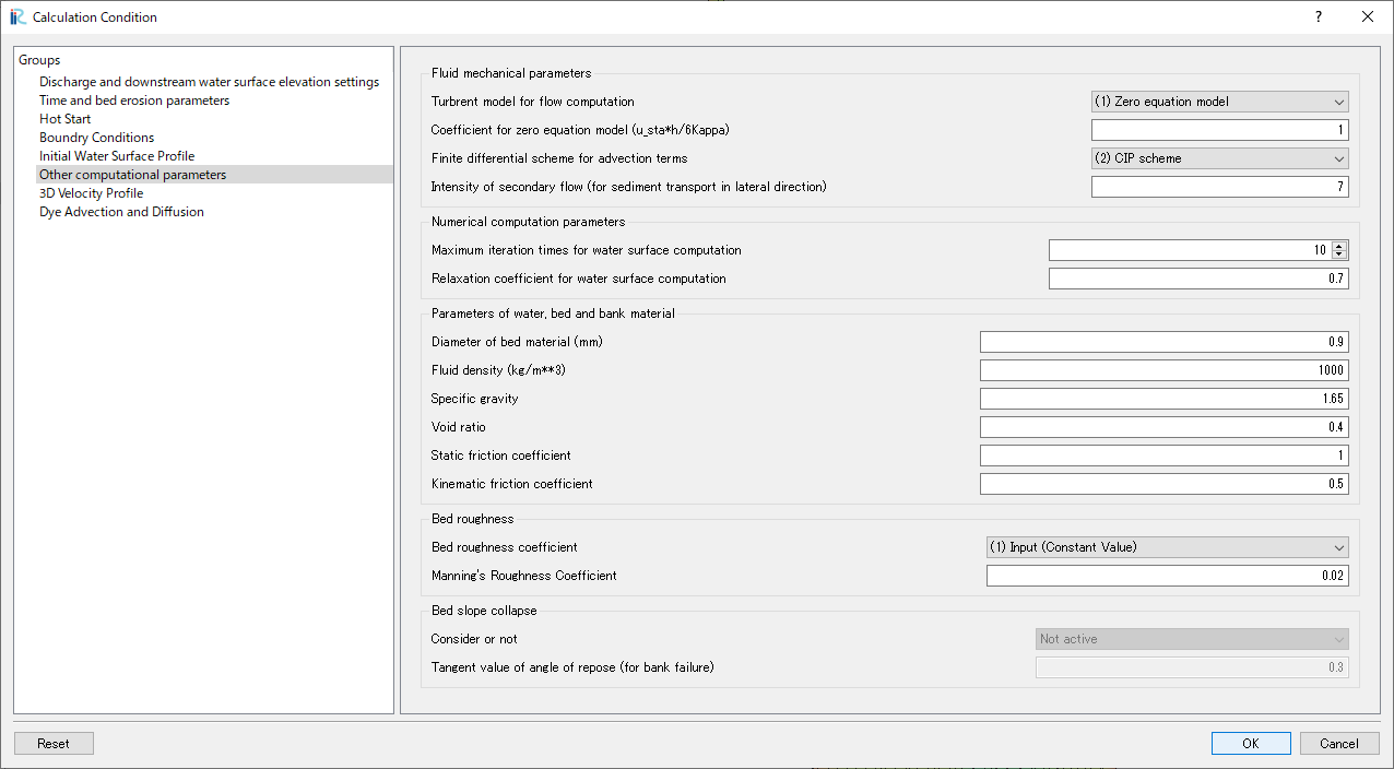
Figure 158 :Other computational parameters
Set “3D Velocity Profile” as shown in the figure Figure 159 , and click [OK] to exit.
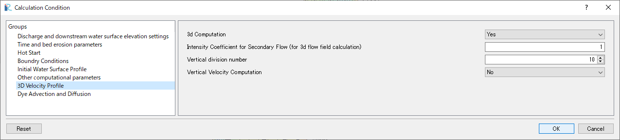
Figure 159 :3D Velocity Profile Settings
Launch Computation
From the menu bar, select [Simulation] and [Run].
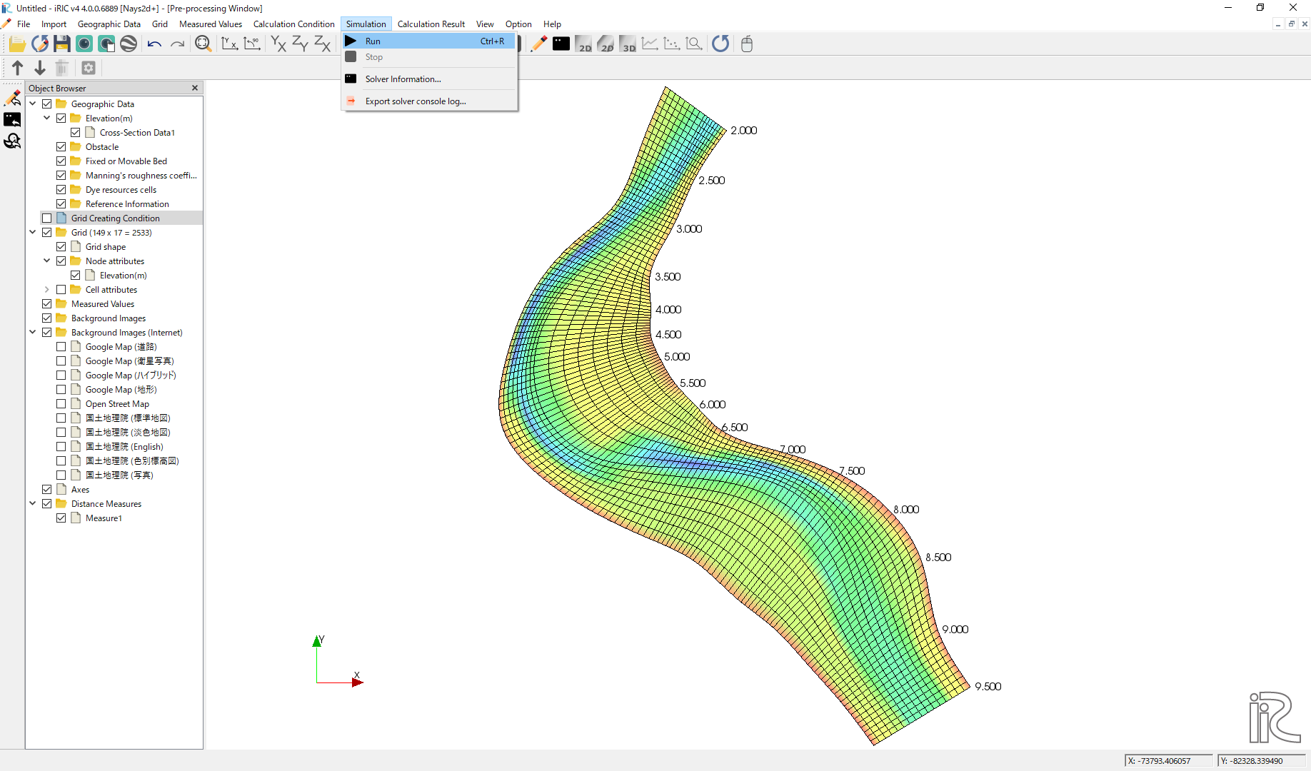
Figure 160 :Launch Simulation(1)
Answer [Yes(Y)] when you asked [Save the project?] as Figure 161
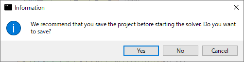
Figure 161 :Launch Simulation(2)
Simulation starts. Figure 162
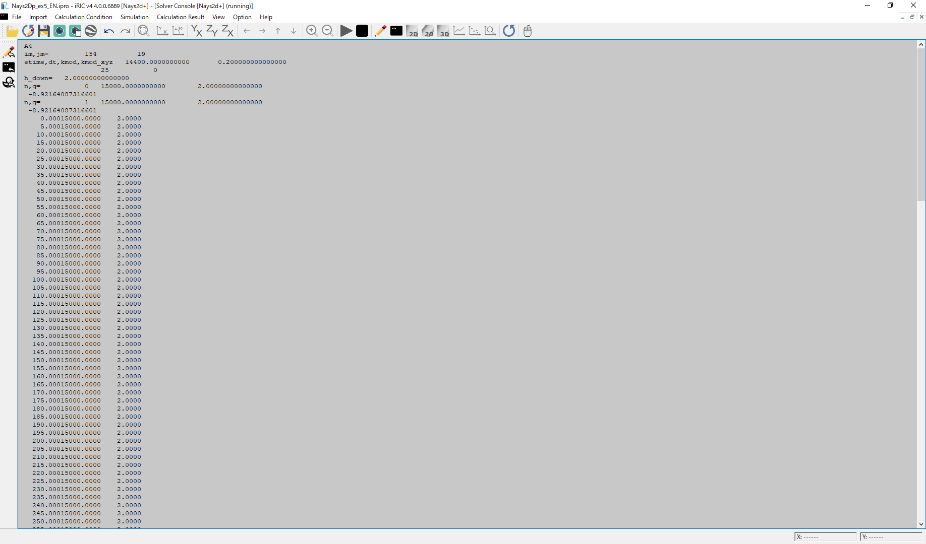
Figure 162 :Launch Simulation(3)
Click [OK] when the message [The solver finished calculation] as Figure 163
Figure 163 :Calculation finished
Display Computational Results
After the companion finished, form the main menu, by selecting [Calculation Results] and [Open new 2D Post-Processing Window], a new Window appears as Figure 164 .
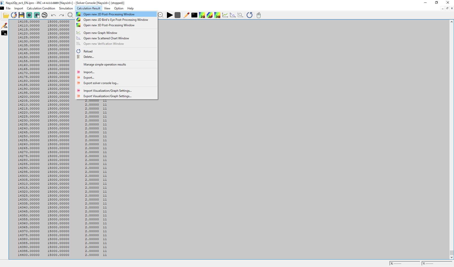
Figure 164 :2D Post-Process Window
Depth
In the object browser, put the check marks in “Scalar (node)” and “Depth[m]”, right-click and select “Properties”. The “Scalar Setting” window Figure 165 appears.
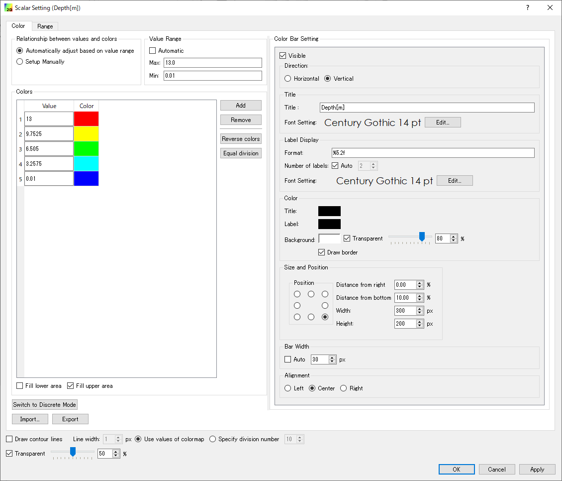
Figure 165 :Scalar Setting
Set the values as shown in Figure 165, and click [OK], then Figure 166 appears.
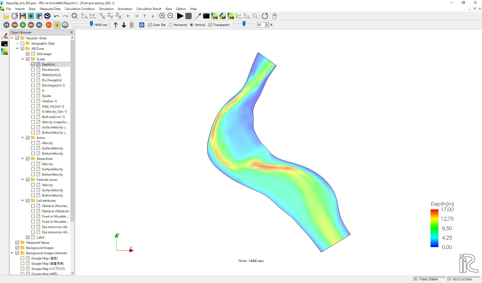
Figure 166 : Depth Plot
Display Background Image
Background images can be imported from Internet resources by the method described in the previous section. After setting the property of the coordinate system, put check marks in a box in front of [Background Images(Internet)] and one of the items listed below, e.g., [Google Map (Satellite Image)], the background image is imported and shown as Figure 167
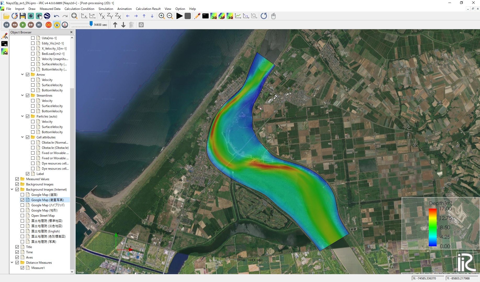
Figure 167 :Background Image Import Complete
Particle Animations
Particle animations can be played by the same procedure with the previous section. Figure 168 shows the particle animation using the depth averaged velocity, Figure 169 shows the particle animation using the surface velocity, and Figure 170 shows the particle animation using the bottom velocity.
Figure 168 :Particle movement by depth averaged velocity
Figure 169 :Particle movement by surface velocity
Figure 170 :Particle movement by bottom velocity
Google Earth Output
From the main menu bar, select [File], [Continuous Snapshot /Movie/Google Export] as Figure 171
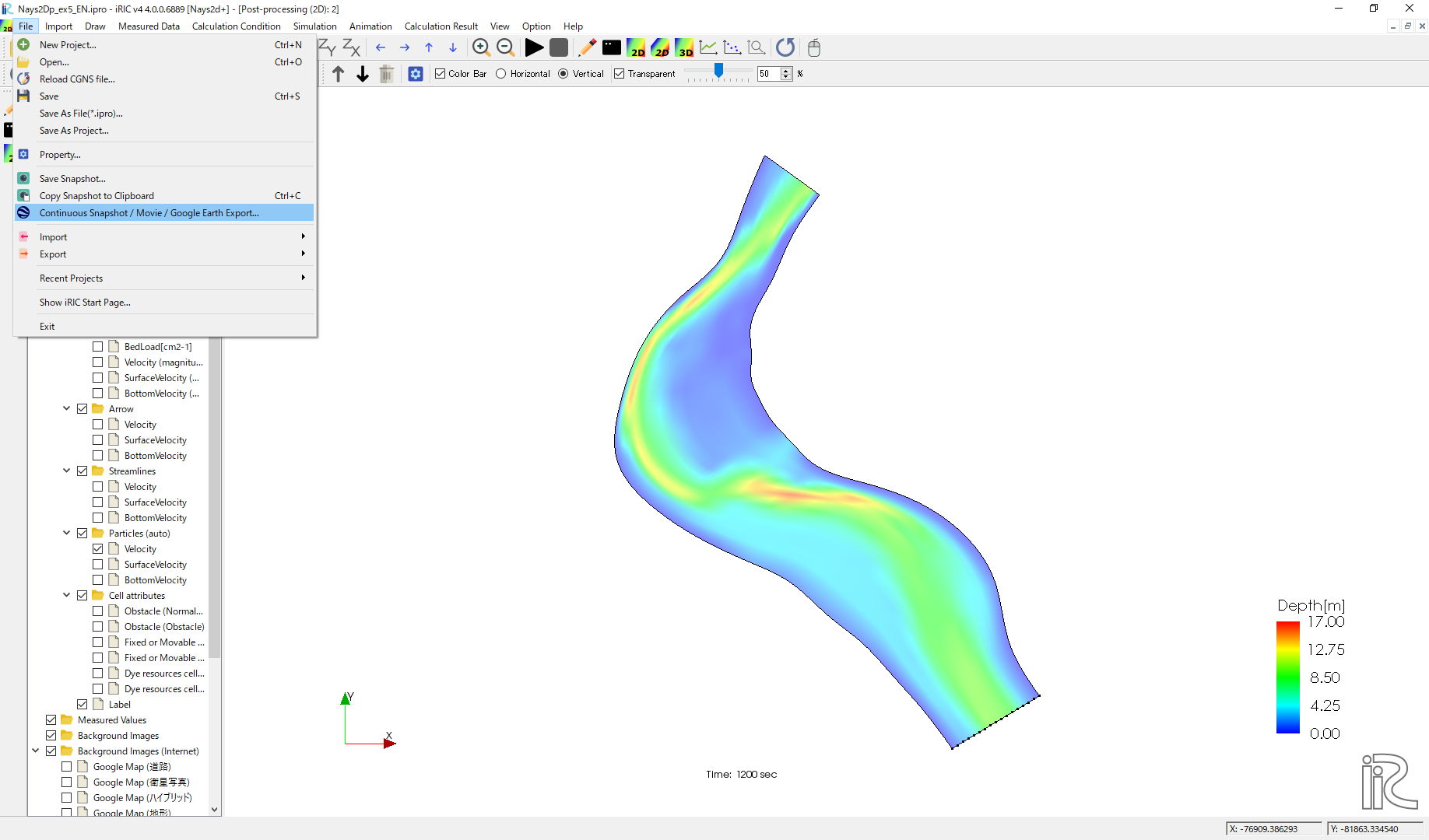
Figure 171 :Animation Settings(1)
Chose [Next(N)] in Figure 172
Figure 172 :Animation Settings(2)
Chose [Next(N)] in Figure 173
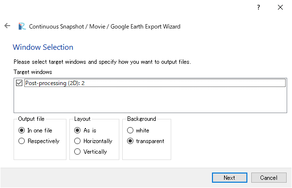
Figure 173 :Animation Settings(3)
Chose [Next(N)] in Figure 174
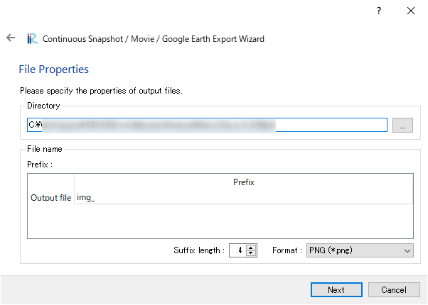
Figure 174 :Animation Settings(4)
Put check mark at [Output movie files], and click [Next(N)] in Figure 175
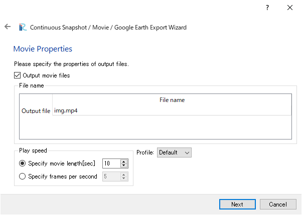
Figure 175 :Animation Settings(5)
Set values as Figure 176 and click [Next]
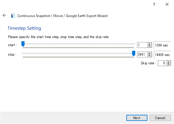
Figure 176 :Animation Settings(6)
Put check mark at [Output to the Google Earth], click [Next] in Figure 177
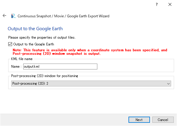
Figure 177 :Animation Settings(7)
click [Finish] in Figure 178
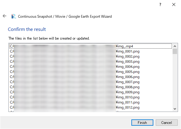
Figure 178 :Animation Settings(8)
Then a file “output.kml” is generated. You can now start playing by double clicking the “output.kml” as Figure 179

Figure 179 :Google Earth Animation