[計算例 5] 下流端水位の上下により蛇行水路内を遡上・流下する塩水楔

感潮河川では，潮の干満により河口水位が上下に振動し，これによって海水(塩水)が河川に侵入および， 流下を繰り返す．河川の水理条件によっては楔状の塩淡境界が河道内を移動する． ここでは，単純なSine Genrlated Curve内を行き来する塩水楔のシミュレーションを行う．

計算格子の生成

計算格子の作成はNays3dv専用の格子生成ツールを用いる． Figure 71 で[Nays3dv用格子生成ツール]を選択し．[OK]をクリックする．

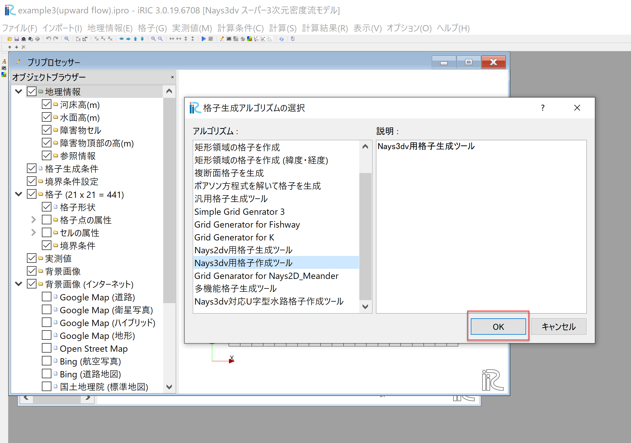
Figure 71 : 格子生成アルゴリズムの選択

「格子生成」ウィンドウが現れるので，[計算領域(流路)形状]を選び， 流路形状は[Sine Generated曲線]をその他の流路形状パラメーターは下の Figure 72 で赤囲いの部分を設定する．

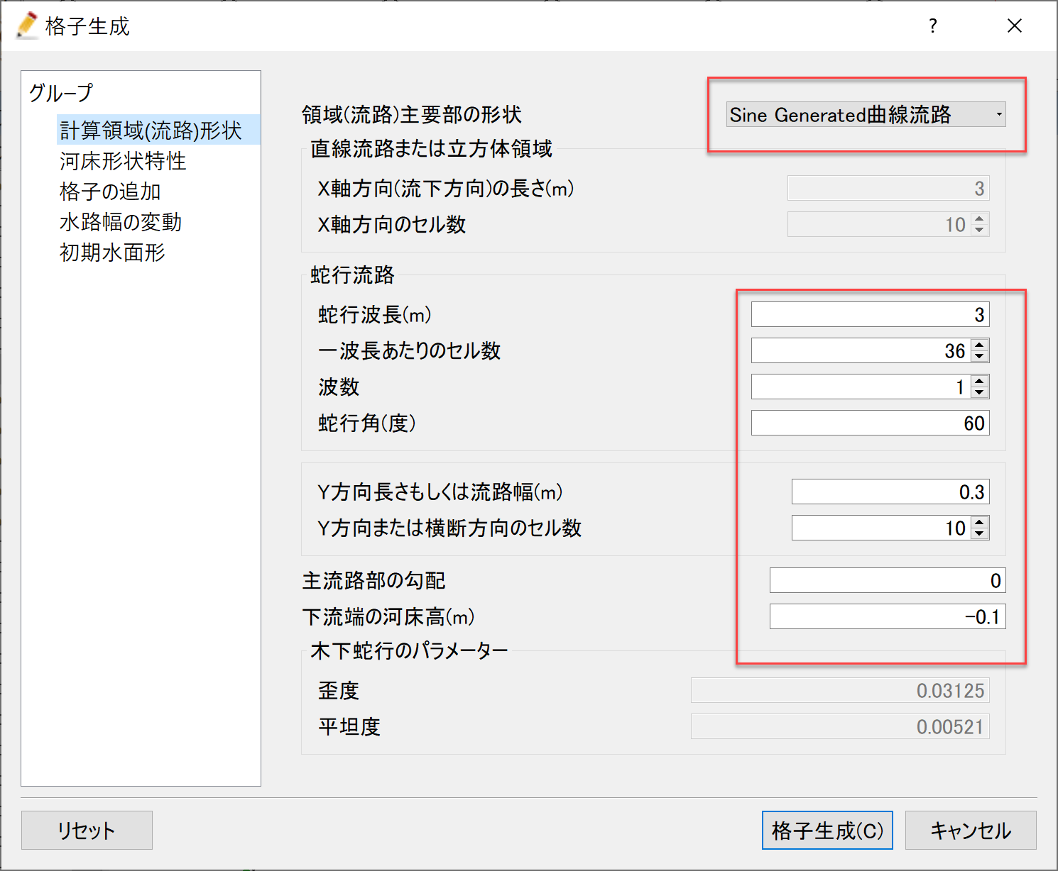
Figure 72 : 格子生成: 計算領域(流路)形状

次に，「格子の追加」を選ぶ．上下流に直線部を追加するので， 下図 Figure 73 で赤囲いの部分を設定する．

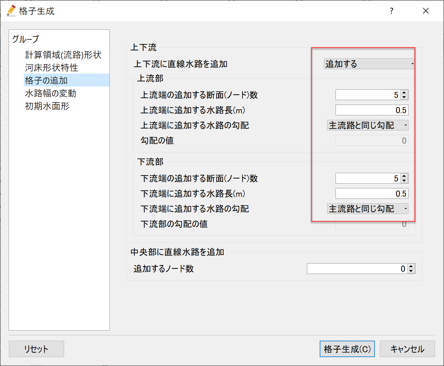
Figure 73 : 格子生成： 格子の追加

最後に，初期水面形を選ぶ． 初期水位は水平とするので，下の 下図 Figure 74 で赤囲いの部分を設定すし，最後に，[格子生成]をクリックすると，格子が生成される．

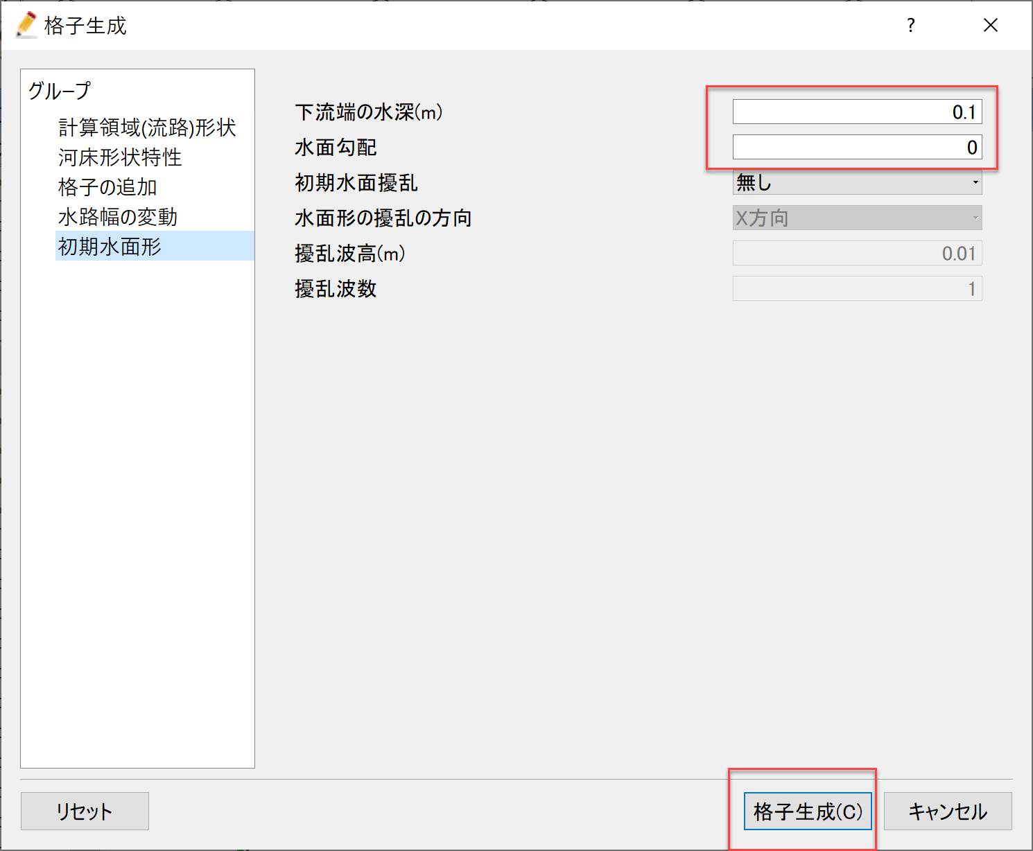
Figure 74 : 格子生成： 初期水面形

Figure 75 が現れ，「マッピングしますか？」と聞かれるので， [はい(Y)]を選択すると，格子生成が完了する．

Figure 75 : マッピング

「プリプロセッサー」ウィンドウに蛇行流路の格子が現れたら，オブジェクトブラウザーで [境界条件設定]→[濃度境界条件の追加]を選び( Figure 76 )，

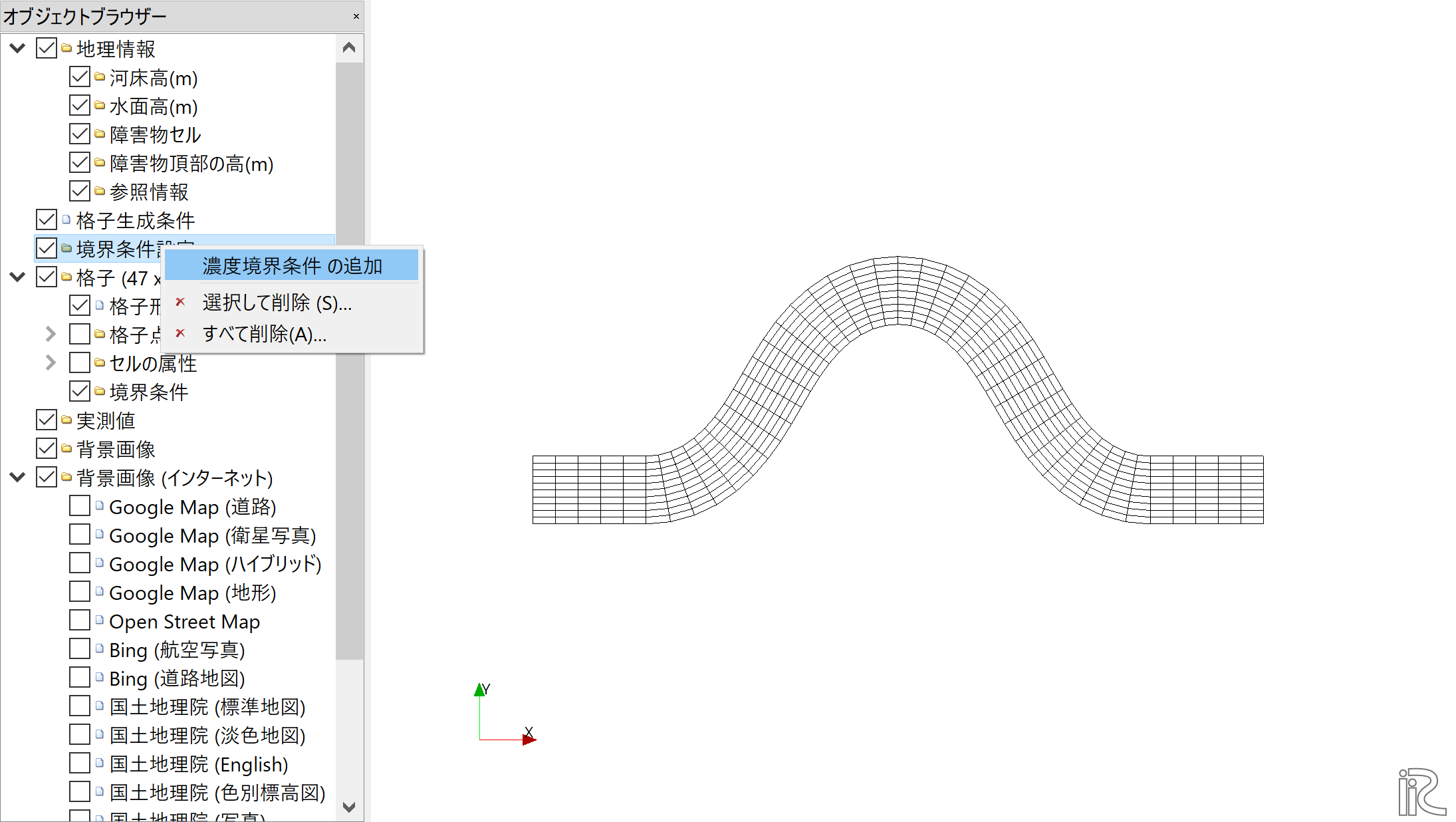
Figure 76 : プリプロセッサー：濃度境界条件の追加

下図 Figure 77 のように，下流端の断面を囲うようにクリックして「濃度境界を与える辺」を指定し， 最後に[Enter]を押す．

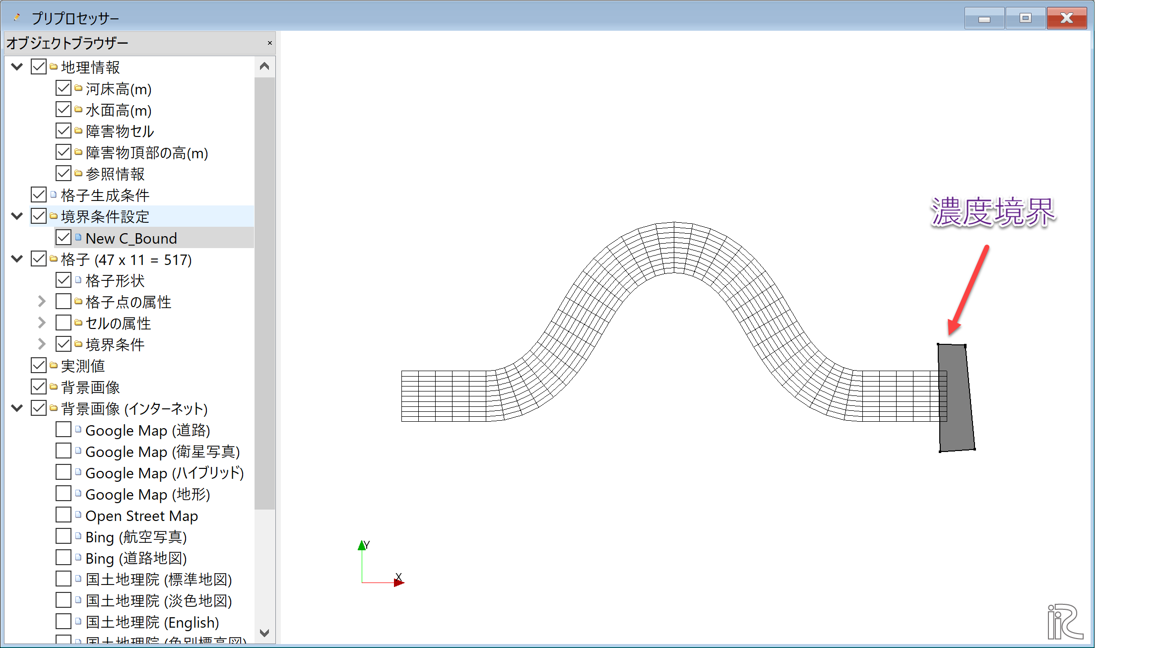
Figure 77 : プリプロセッサー：濃度境界条件の追加

下図 Figure 78 が現れるので，「境界条件濃度を」[0.03]に， 濃度境界条件を与える高さ(m)を[-0.05]とする．本計算例では下流端の水位が初期で0m, 河床高が-0.1mとした ので，「濃度境界条件を与える高さ」を[-0.05]mとすることによって，-0.05mの高さまでが境界条件で 海水となることを表す．設定が終了したら[OK]を押す．

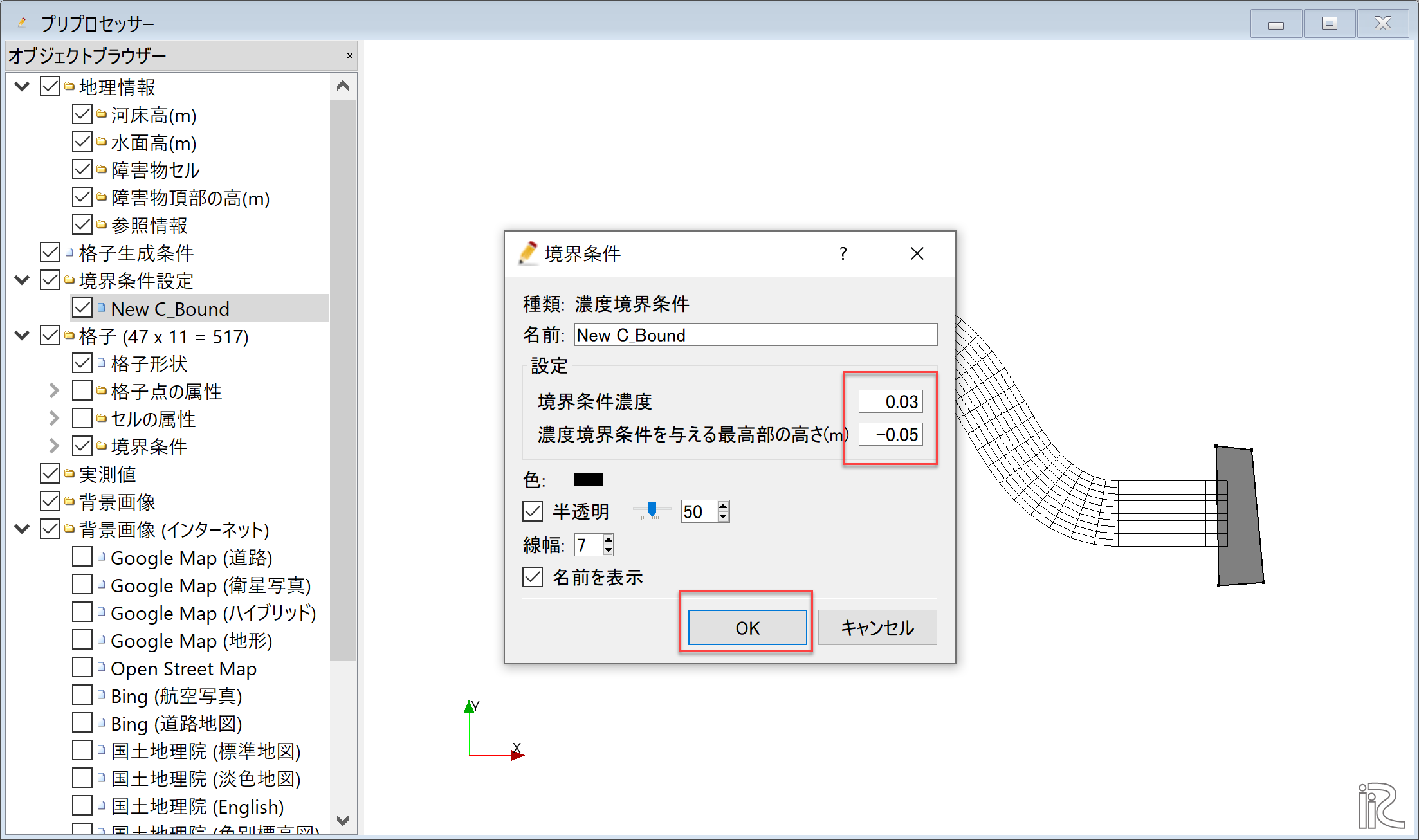
Figure 78 : プリプロセッサー：濃度境界条件

計算条件の設定

メニューバーから[計算条件]→[設定]を選ぶと「計算条件」入力用のウィンドウが表示される Figure 79

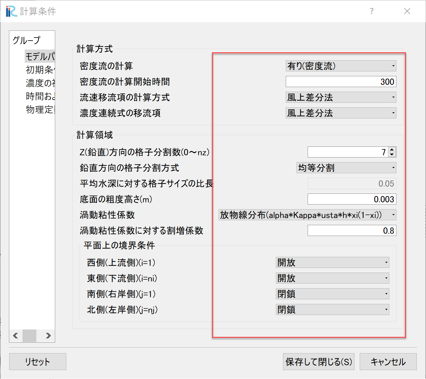
Figure 79 : 計算条件：モデルパラメータ

「計算条件」ウィンドウ Figure 79 の「モデルパラメータ」は図の赤で囲った部分を設定する． 本計算は密度流なので，「密度流の計算」を[有り]に, ここでは「差分式」を[風上差分]，「鉛直方向の分割数」は [7] とする．流れの渦動粘性係数は流速の対数分布に対応する[放物線分布]とする．

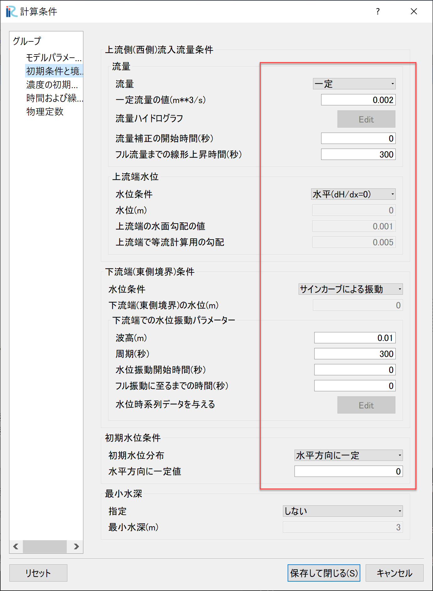
Figure 80 : 計算条件：濃度の初期条件と境界条件

「計算条件」の「初期条件と境界条件」は，河川流量は一定，下流端は周期的な振動とするので， Figure 80 の赤囲いのように設定する．

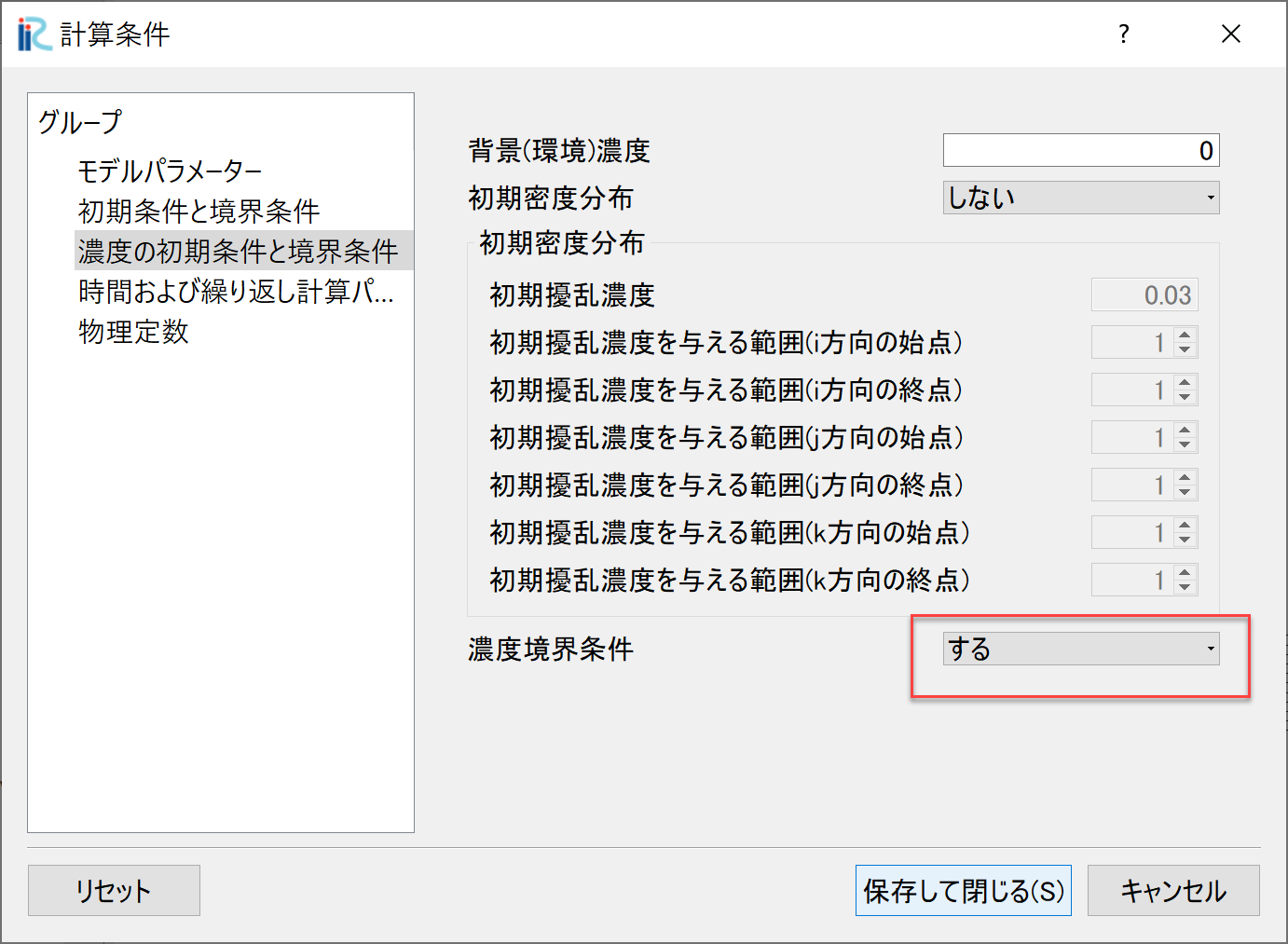
Figure 81 : 計算条件：時間およに繰り返し計算パラメーター

「計算条件」の「濃度の初期条件と境界条件」下流端の濃度境界のみ考慮するので， Figure 81 の赤囲いのように設定する．

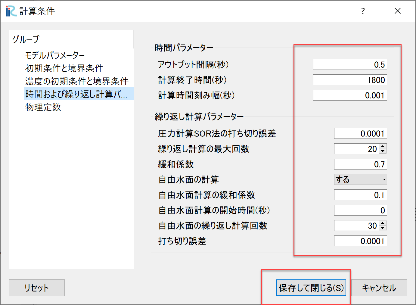
Figure 82 : 計算条件：時間およに繰り返し計算パラメーター

「計算条件」の「時間およに繰り返し計算パラメーター」は， Figure 82 の赤囲いのように設定する．下流端の水位変動が上流に及ぶ ことによる塩水楔の移動なので，自由水面の計算は[する]に設定する．

設定が終了したら，[保存して閉じる]を押す．

計算の実行

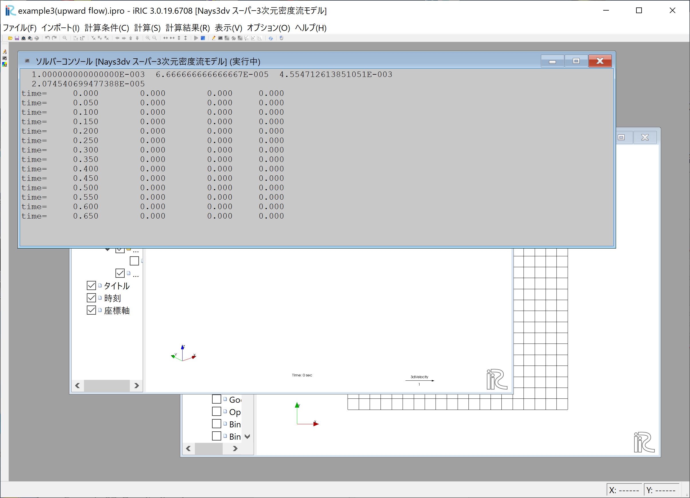
Figure 83 :計算実行中の画面

[計算]→[実行]を指定すると，Figure 83 のような画面が現れ計算が始まる．

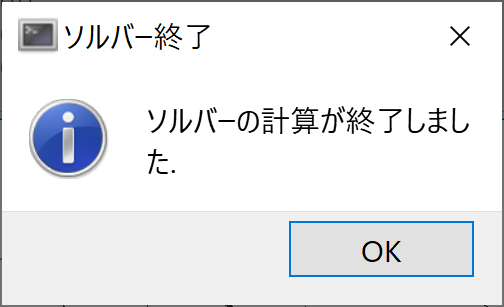
Figure 84 :計算の終了

計算が終了すると, Figure 84 のような表示がされる．

計算結果の表示

計算の終了後，[計算結果]→[新しい可視化ウィンドウ(3D)を開く]を選ぶことによって，可視化ウィンドウ(3D)が現れる．

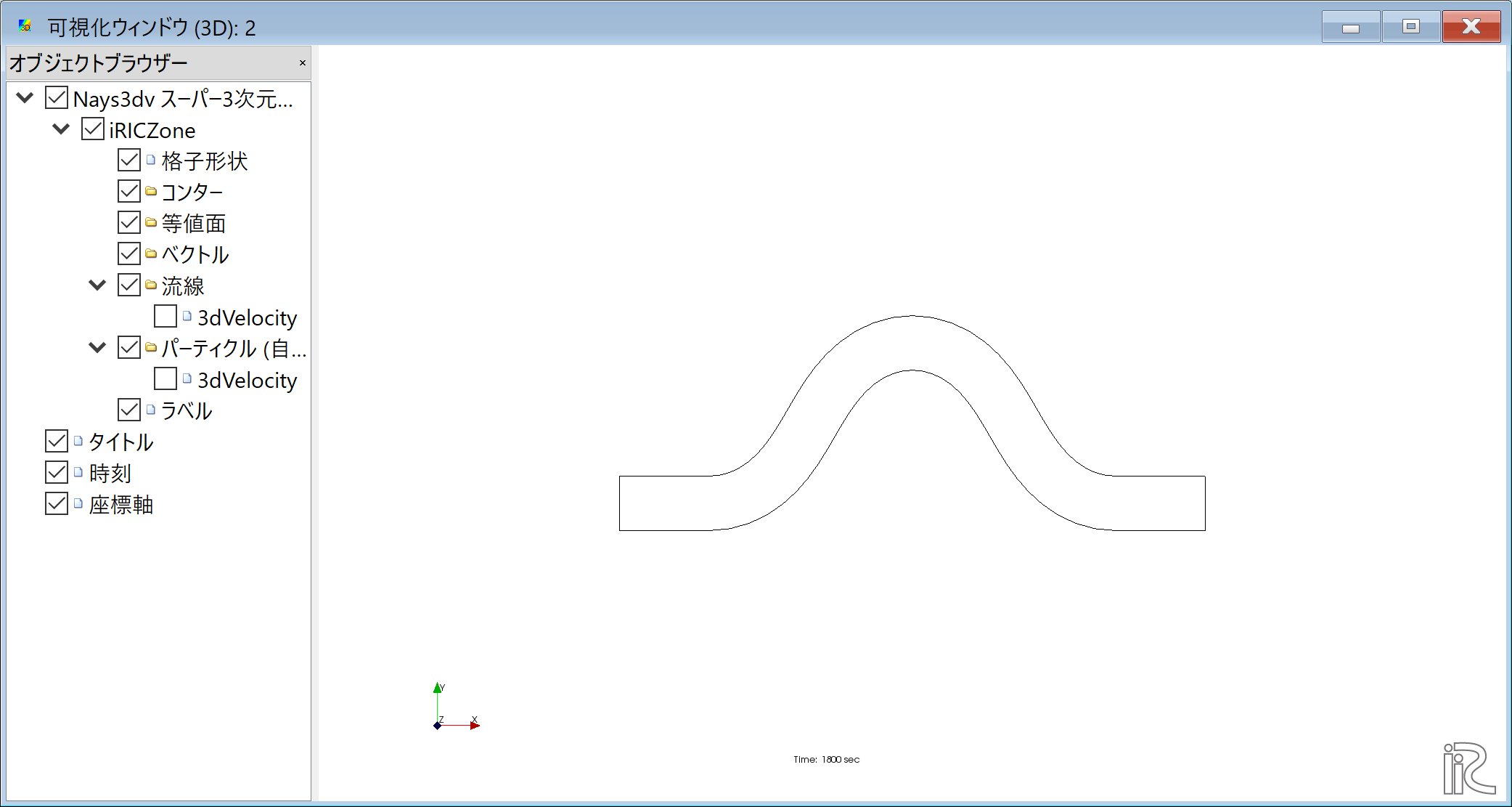
Figure 85 : 計算結果の表示(1)

「Ctrl」ボタンとマウス右ボタンを押しながらマウスを上下左右に動かすことによって， 3次元的な見え方が，また，マウスぼセンターダイヤを回すことにより， Figure 86 のような 拡大・縮小が可能となっている．

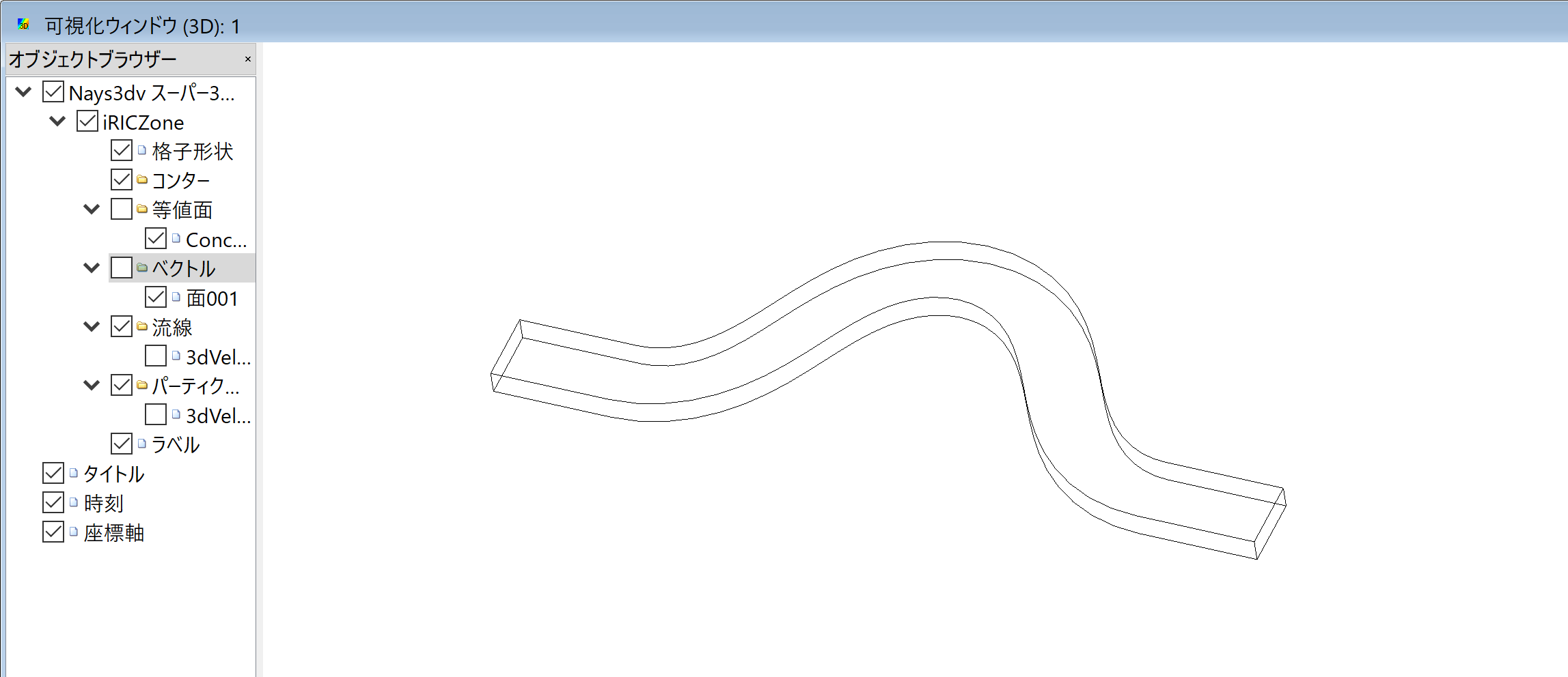
Figure 86 : 3D格子の回転・移動・拡大・縮小

Z方向の表示を拡大したい場合は，メニューバーから[表示]→[Z方向の倍率]を選んで，( Figure 87 )

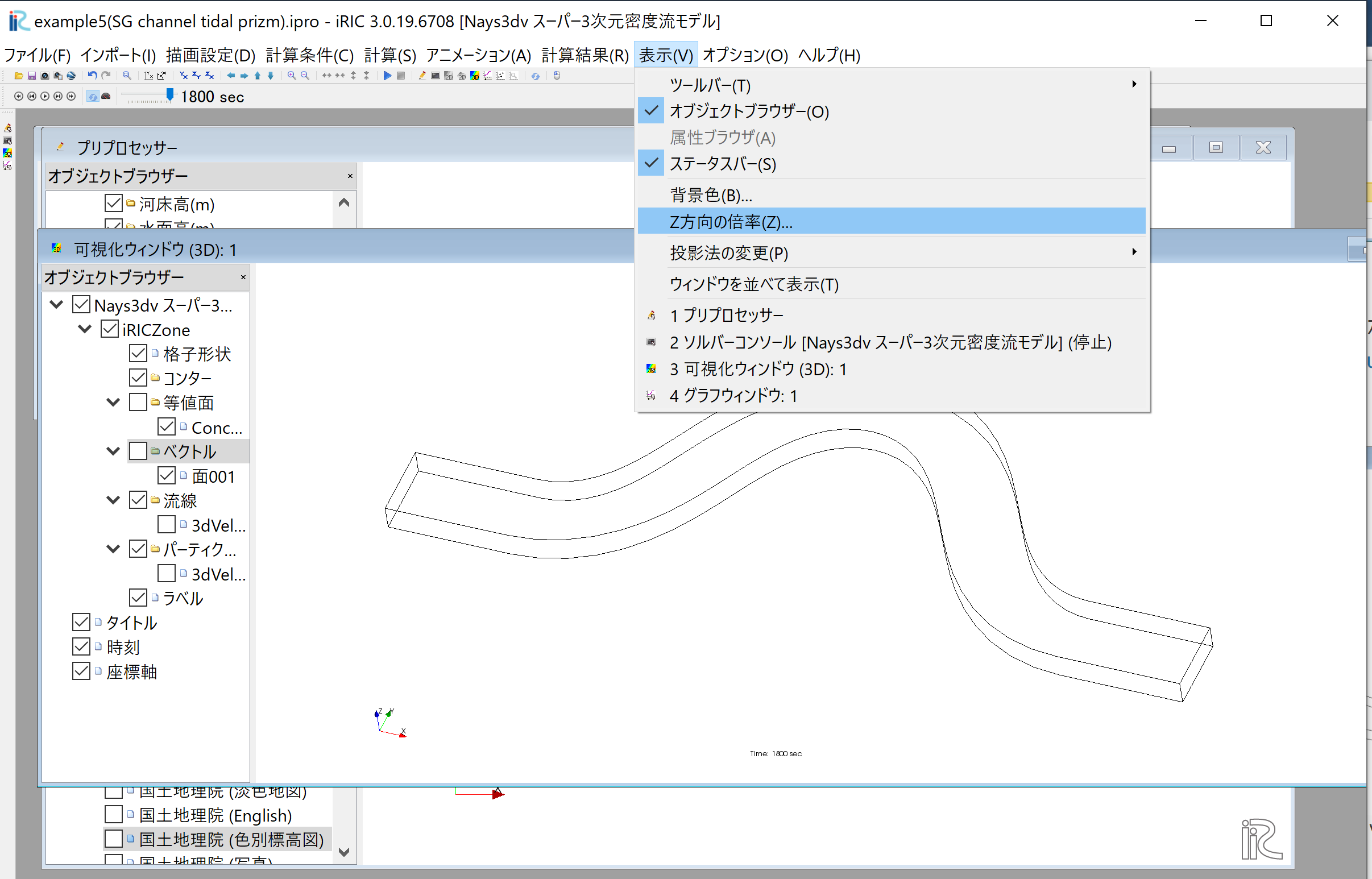
Figure 87 : Z方向の倍率

任意の倍率(ここでは2)を入力して，[OK]を押す．( Figure 88 )

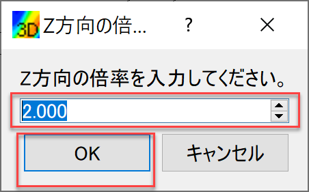
Figure 88 : Z方向の倍率の指定

ベクトル表示の設定

オブジェクトブラウザーで，[ベクトル]を右クリックして，[プロパティ]をクリックすると， 「ベクトル設定」ウィンドウ Figure 89 が現れる．

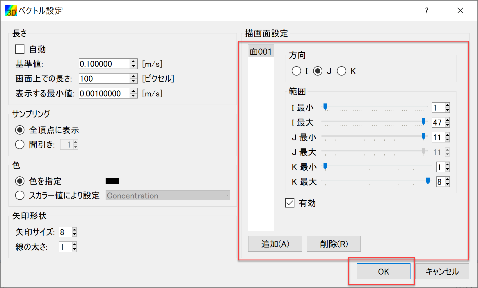
Figure 89 : ベクトルの設定

Figure 89 のようにベクトルに関する各パラメータを設定し，[OK]ボタンを押す．

等値面表示の設定

オブジェクトブラウザーで，[等値面]を右クリックして，[追加]をクリックすると， 「等値面設定」ウィンドウ Figure 90 が現れる． これを図のように設定して[OK]を押す．

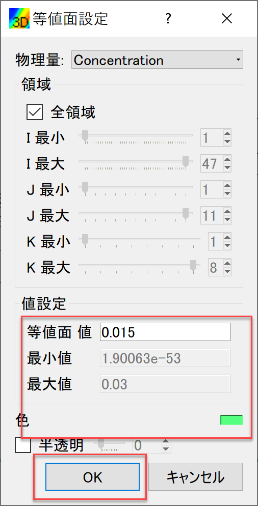
Figure 90 : 等値面の表示

計算結果の表示およびアニメーション

「可視化ウィンドウ(3D)」 Figure 91 でタイムバーをゼロに戻して，[アニメーション]→[開始/停止]で 計算結果をアニメーションで見ることが出来る．

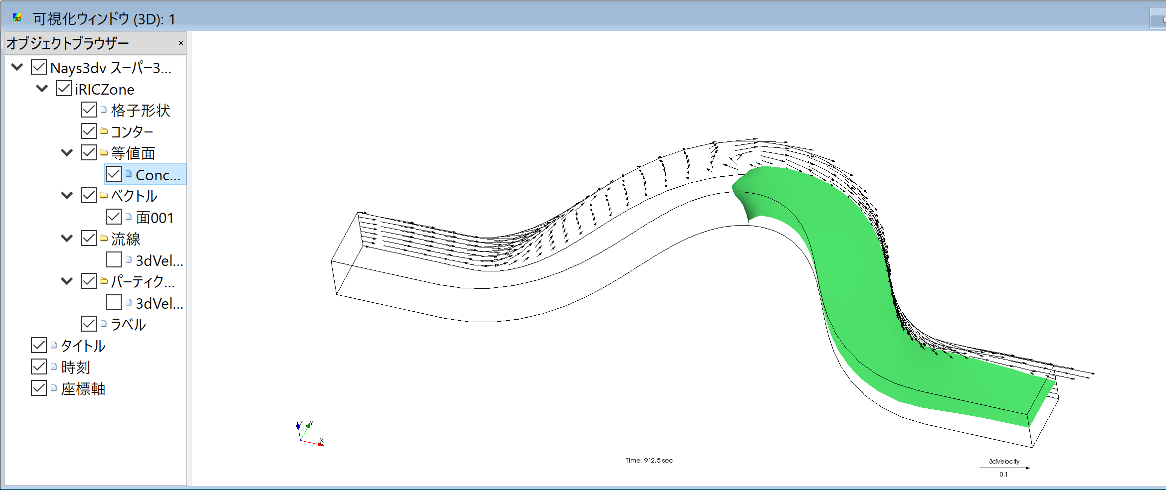
Figure 91 : アニメーション

アニメーションはiRICメインウィンドウ左上にあるプレイボタン等で操作も可能である．Figure 92

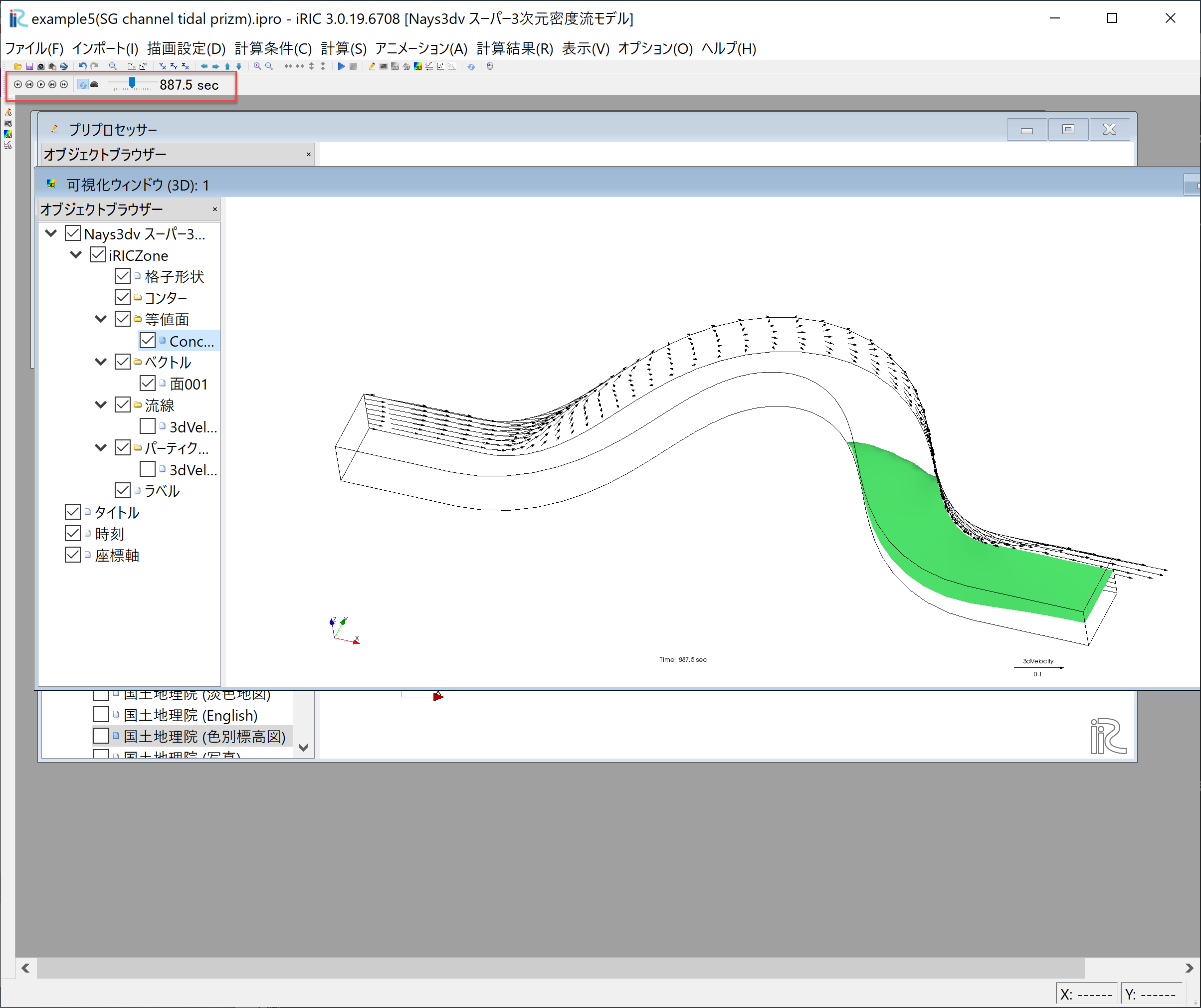
Figure 92 : アニメーション

グラフの表示

下流端水位の時間変化を表示するグラフを作成する． メニューから[計算結果]→[新しいグラフウィンドウを開く]をクリック Figure 93 すると，

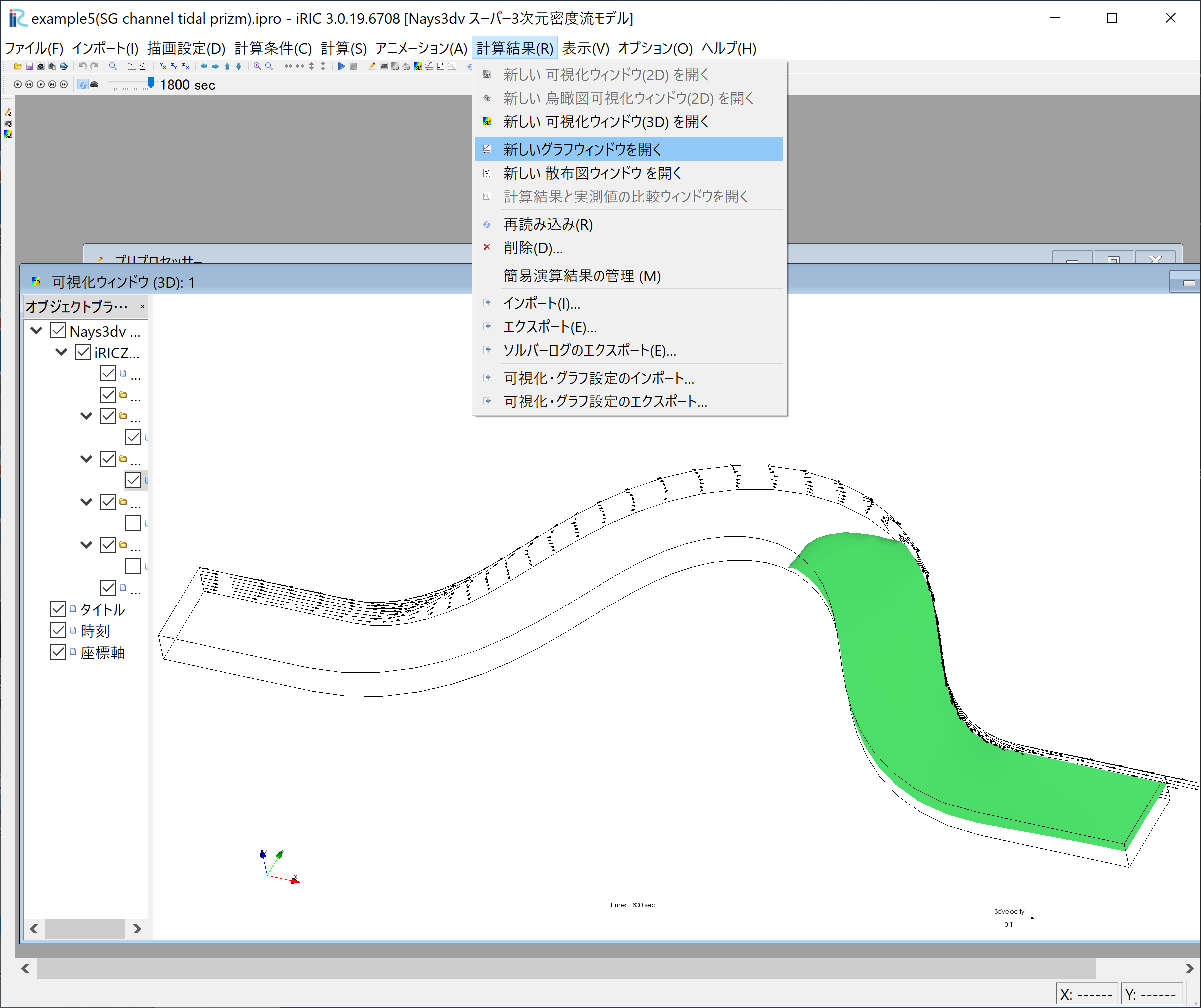
Figure 93 :グラフウィンドウを開く

「データソース設定」のウィンドウ Figure 94 が表示される． 「X軸】に[時刻]を，「計算結果」の「ポイントデータ」に[Dounstream Stage」を指定し， [追加]をクックりっくする．

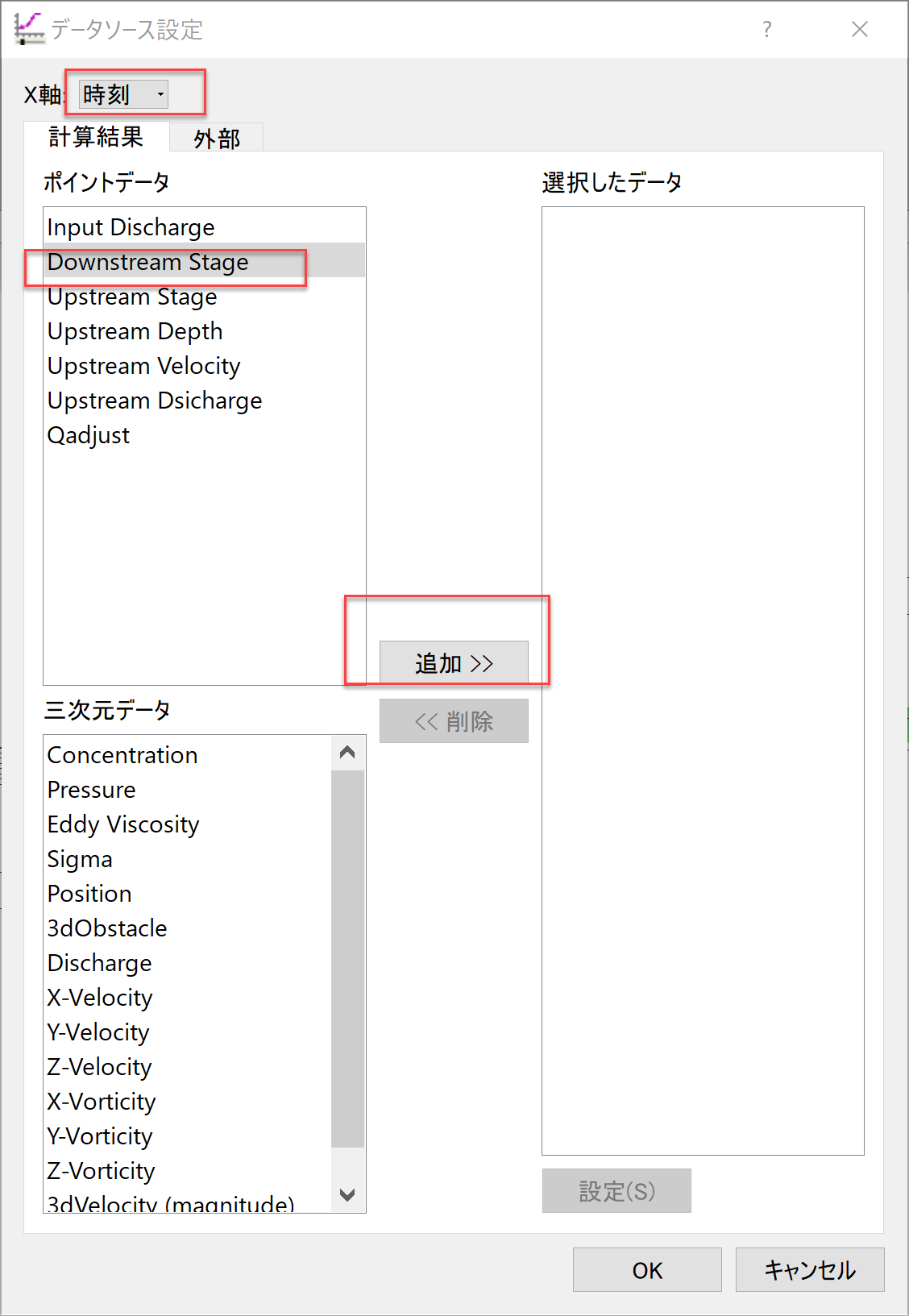
Figure 94 :データソース設定(1)

「選択したデータ」に[Doenstream Stage]が移動するので，[OK]をクリックする. Figure 95

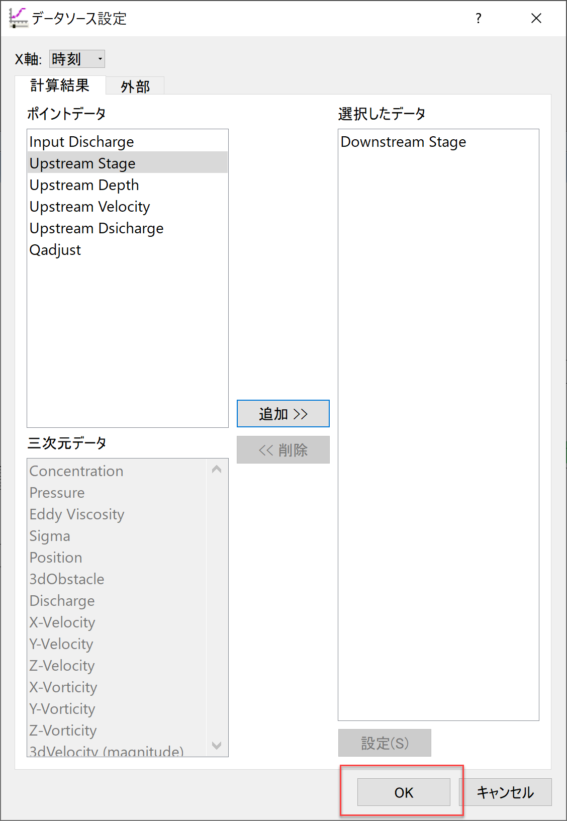
Figure 95 :データソース設定(2)

下流端水位の時間変化グラフ Figure 96 が表示される． Figure 96

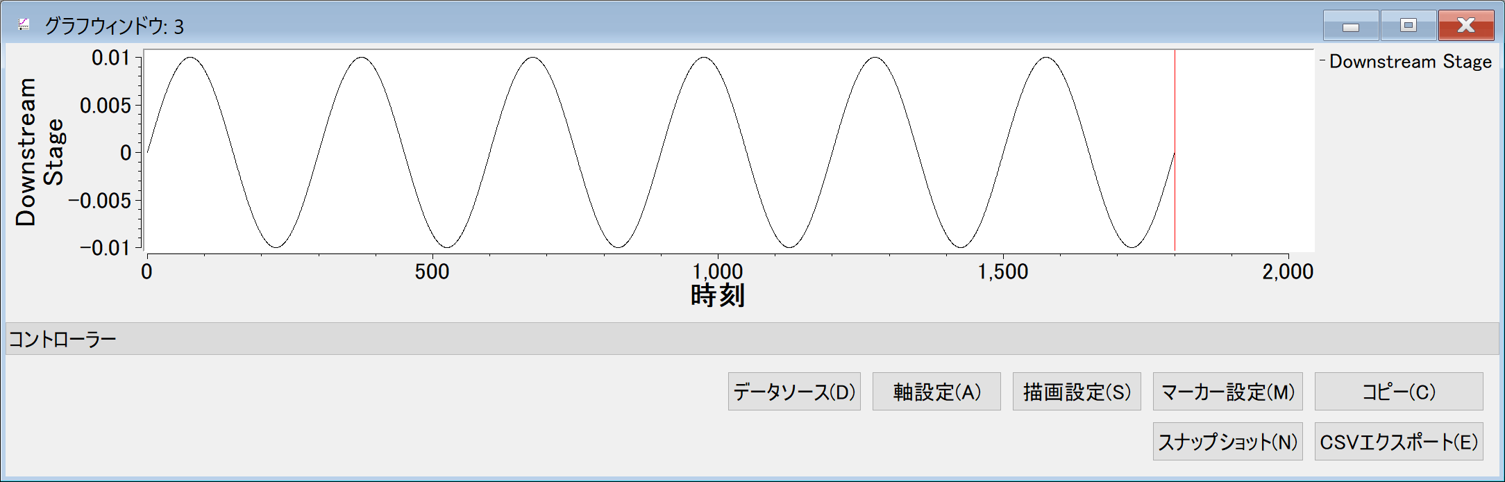
Figure 96 :グラフウィンドウ(下流端水位の時間変化)

アニメーション動画の作成

可視化ウィンドウとグラフウィンドウをいつの画面に入れたアニメーションファイルを作成する． メニューバーから[ファイル]→[連続スナップショット/動画/Google Earth出力]を選ぶ． Figure 97

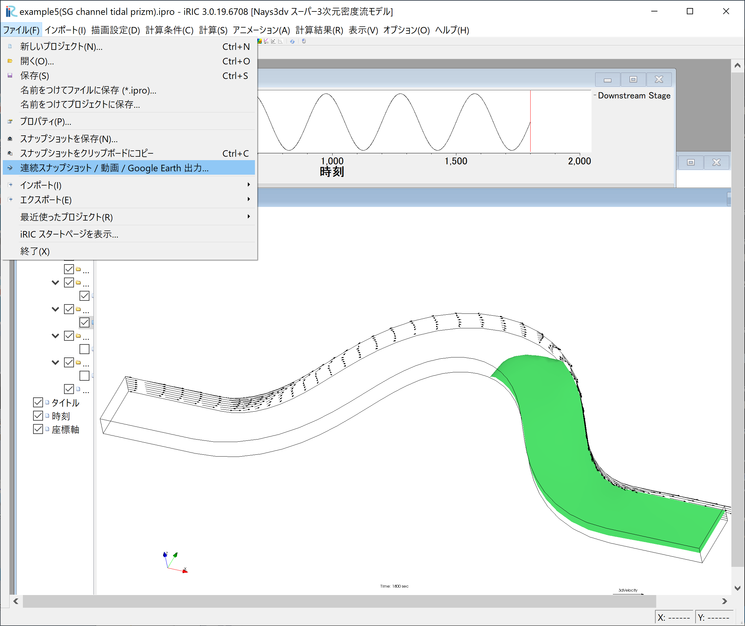
Figure 97 :[連続スナップショット/動画/Google Earth出力]の選択

下図 Figure 98 で[次へ]をクリック

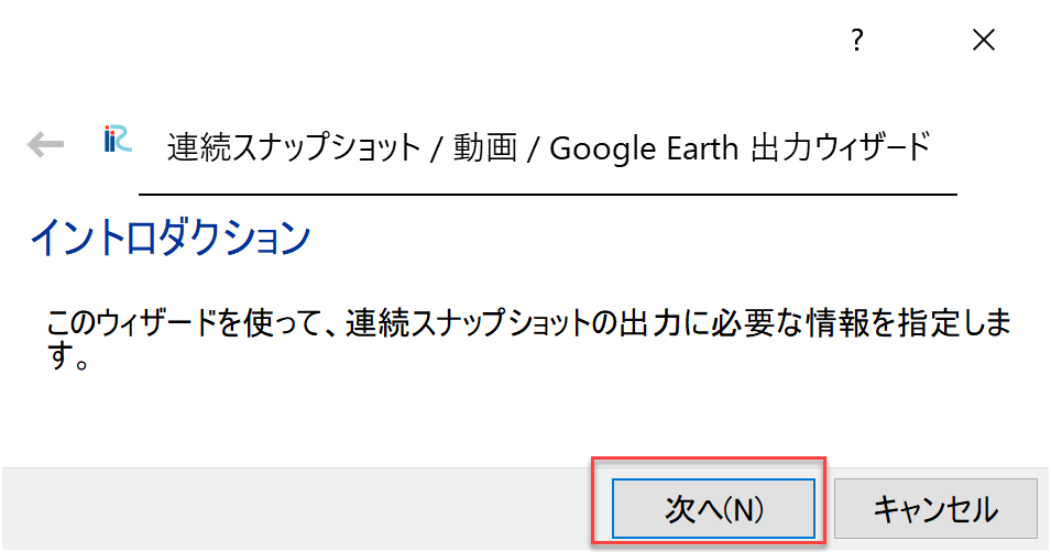
Figure 98 :イントロダクション

下図 Figure 99 で赤囲い部分をチェックして[次へ]をクリック

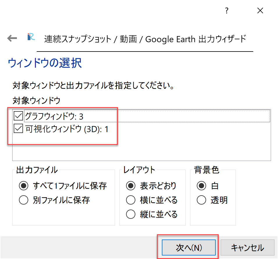
Figure 99 :ウィンドウの選択

下図 Figure 100 で画像と動画の出力フォルダを指定して[次へ]をクリック

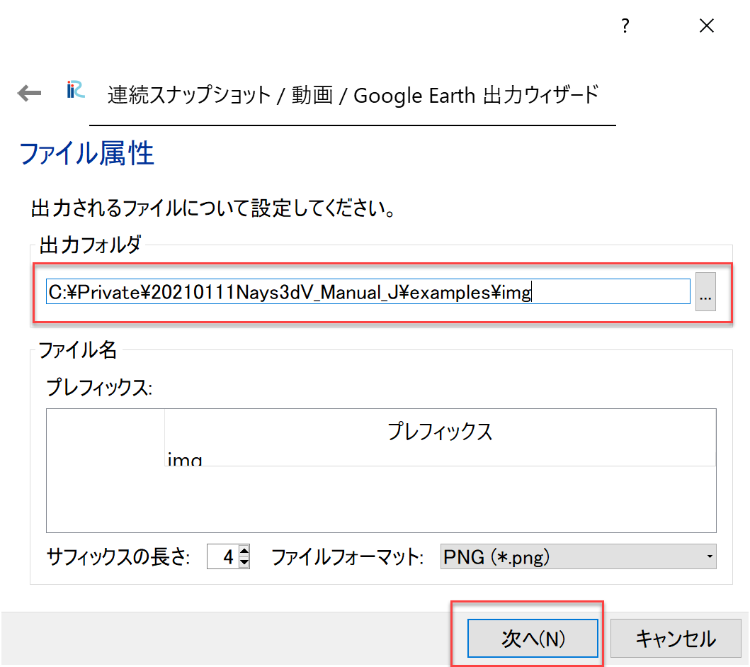
Figure 100 :ファイル属性

下図 Figure 101 で「動画ファイルに出力」をチェック，「動画の長さ」を 10秒にして，[次へ]をクリック

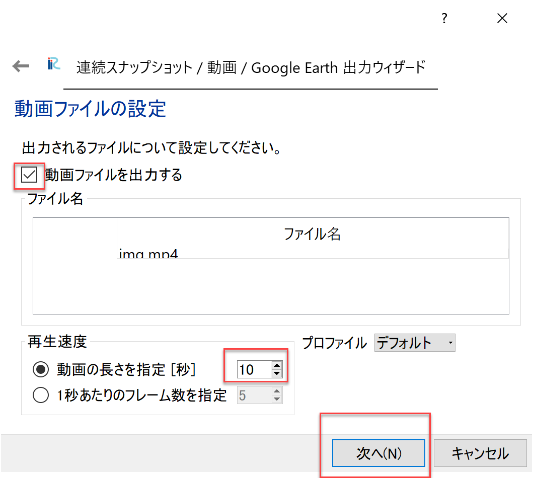
Figure 101 :動画ファイルの設定

下図 Figure 102 で[次へ]をクリック

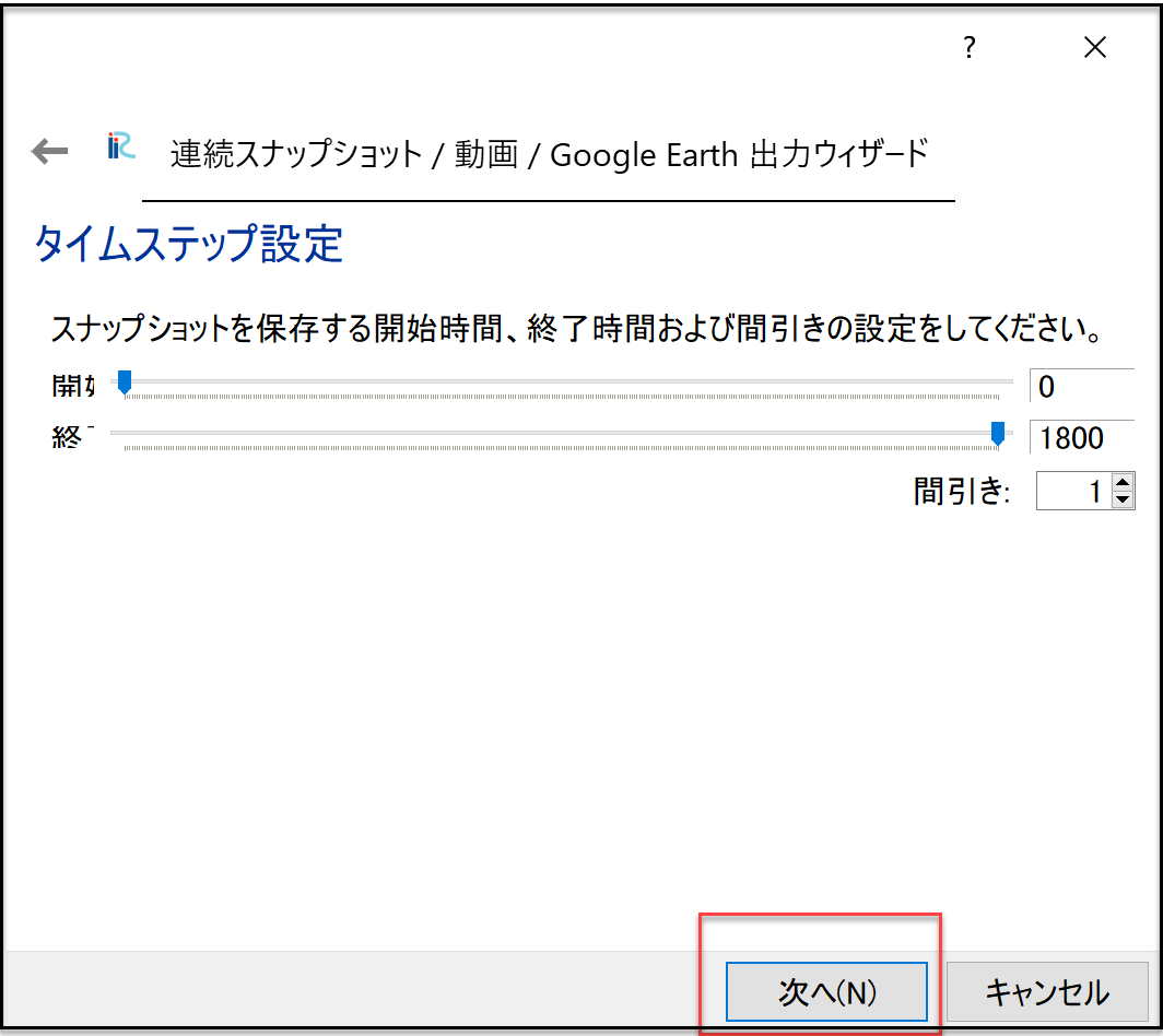
Figure 102 :タイムステップ設定

下図 Figure 103 で[次へ]をクリック

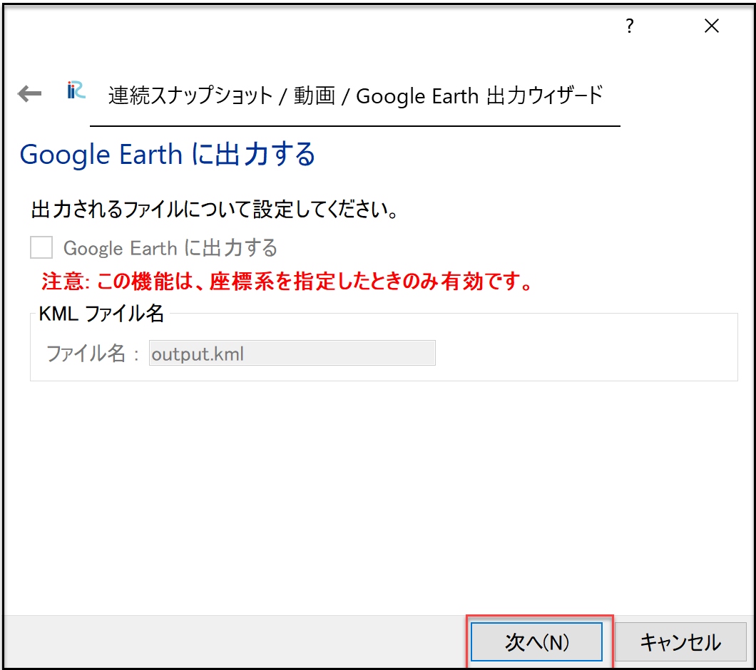
Figure 103 :Google Earth 出力設定

下図 Figure 104 で[完了]をクリック

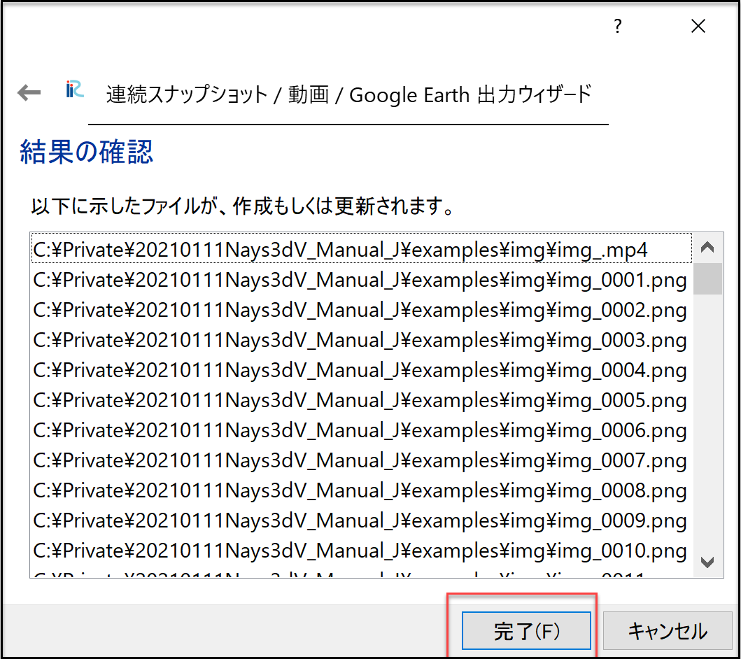
Figure 104 :結果の確認

しばらく待つと，動画ファイルは，で画像と動画の出力フォルダの中の「image.mp4」というファイル名で 作成される．

Figure 105 :計算結果のアニメーション