[計算例 1] 直線水路におけるトレーサーの輸送
Nays2DHによる流れの計算
ソルバの選択
iRICの起動画面から,[新しいプロジェクト]を選ぶと表示されるソルバの選択画面で, [Nays2dh 簡単に3次元流れの計算ができます]を選んで[OK]ボタン押すと,
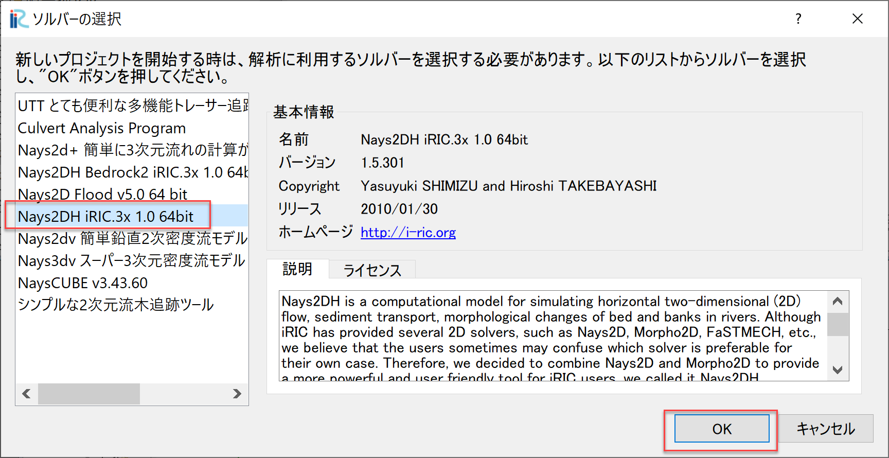
Figure 9 : ソルバーの選択
「無題- iRIC 3.x.xxxx [Nays2DH iRIC3X 1.0 64bit]」と書かれた Windowが現れる.
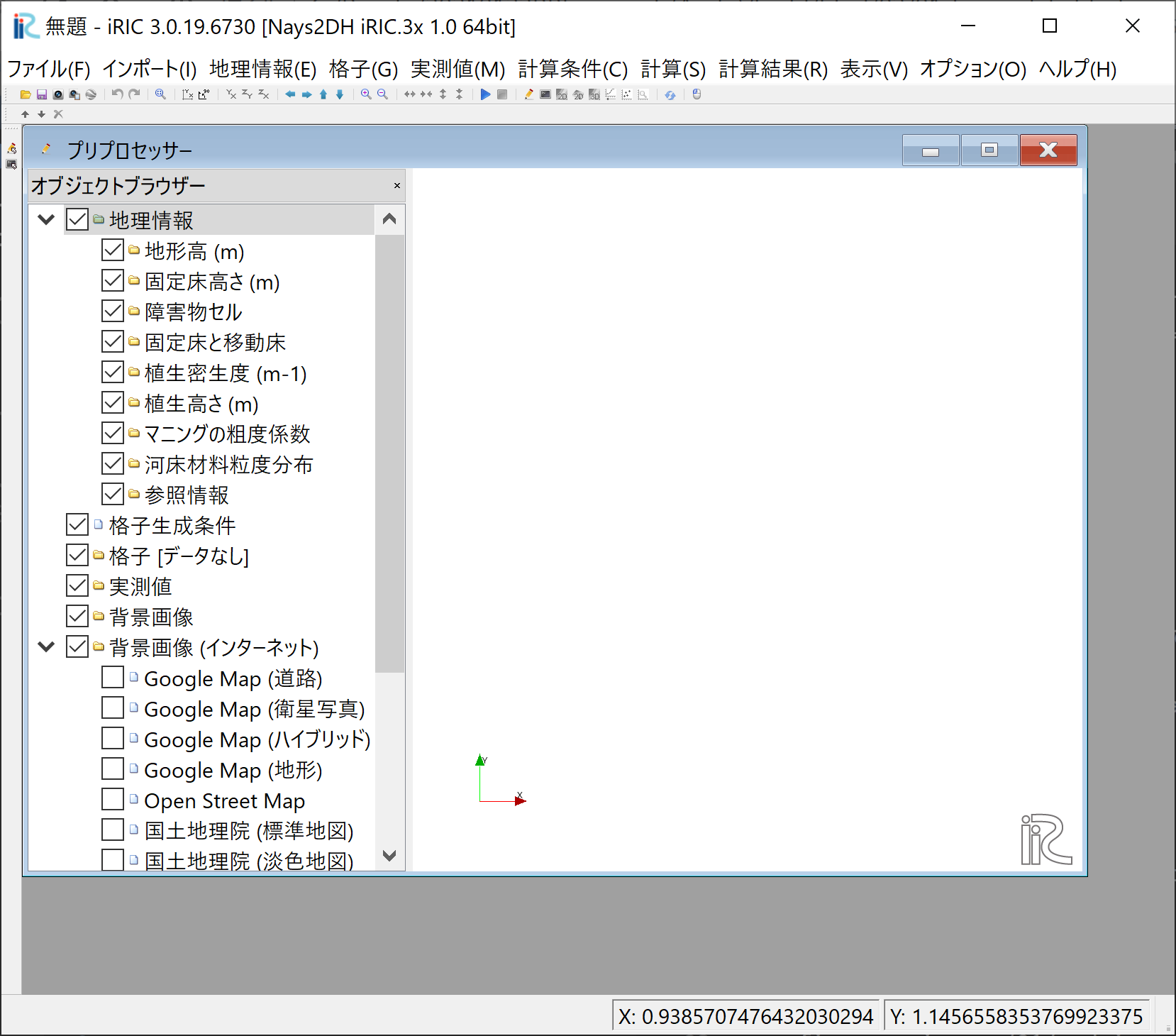
Figure 10 : 無題
計算格子の作成
Figure 10 のウィンドウで,[格子]→[格子生成アルゴリズムの選択]から現れる, 「格子生成アルゴリズムの選択」ウィンドウ で[簡易直線・蛇行生成ツール]を選んで[OK]を押す.
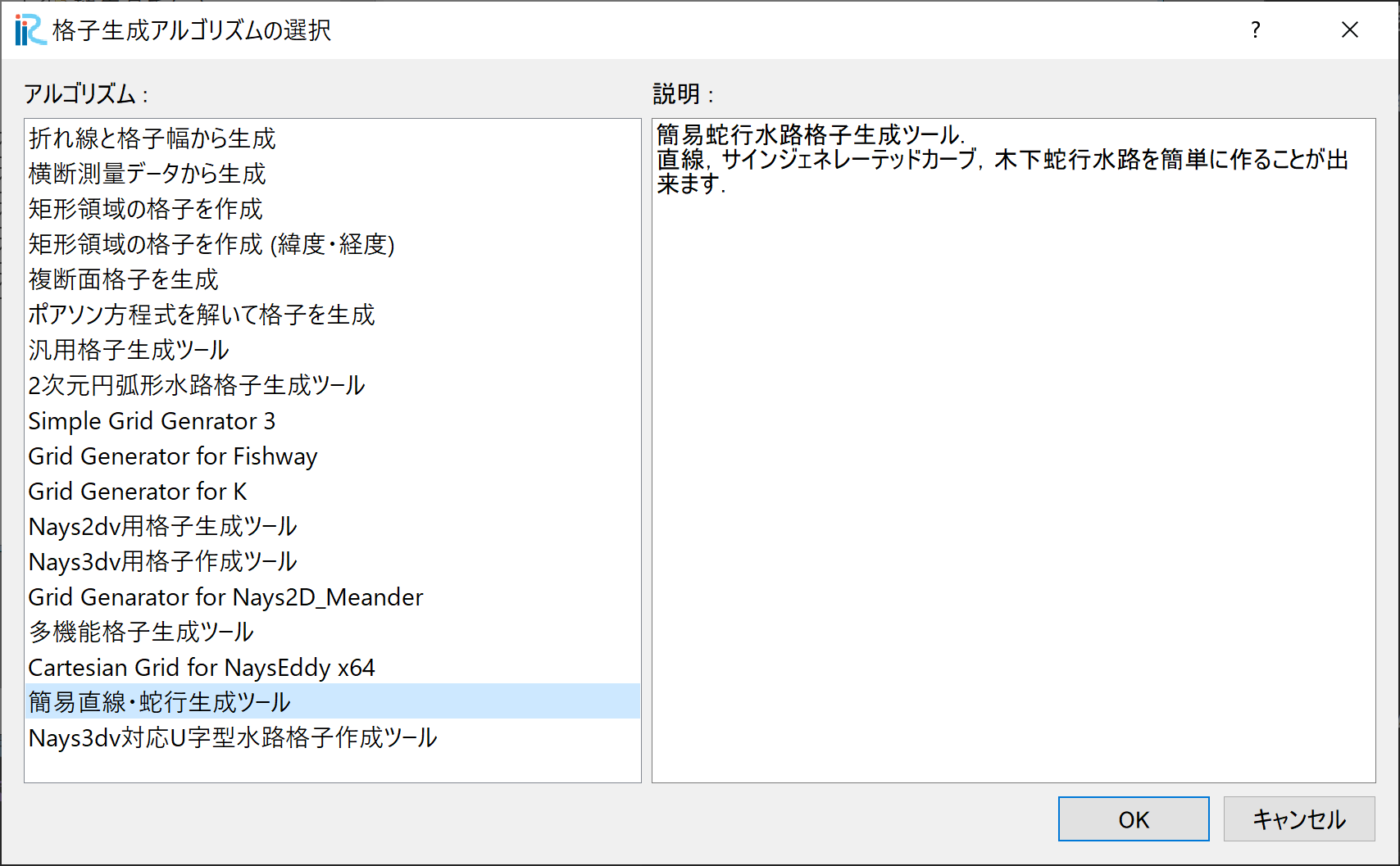
Figure 11 : 格子生成アルゴリズムの選択
Figure 12 の画面で,「水路形状」を選択し, 「水路主要部の形状」を[直線水路],「X方向長さもしくは流下方向延長(m)」を[5], 「X方向の格子数」を[100],「Y方向長さもしくは水路幅(m)」を[0.5], 「Y方向または横断方向格子数」を[20], 「主要部の河床勾配」を[0.005],「下流端の河床高(m)」を[-0.5]に 設定し,他はすべてデフォルトなので,「格子生成」をクリックする.
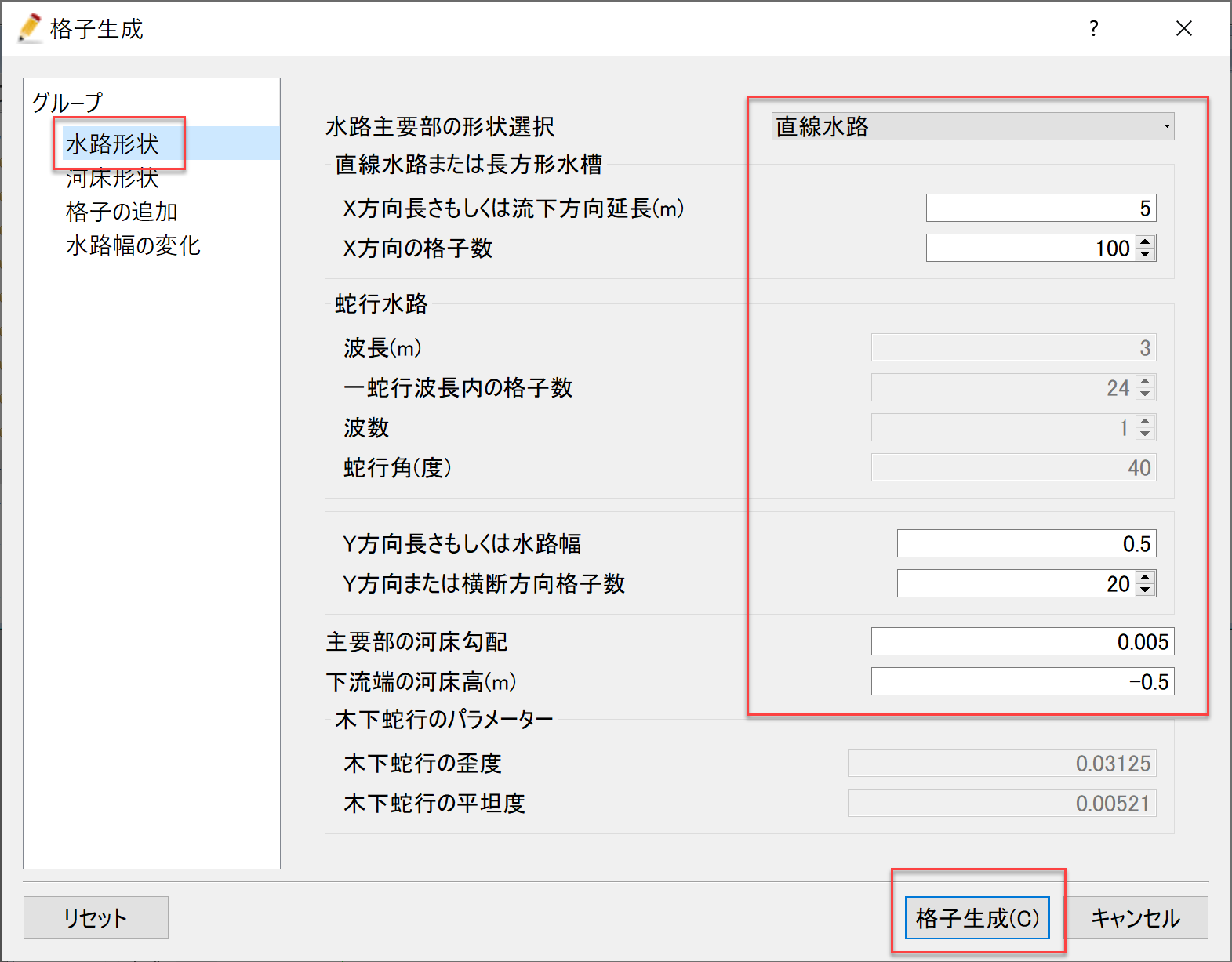
Figure 12 :水路形状
すると,Figure 13 確認ウィンドウが現れるので,[はい(Y)]を押すと格子が生成され, Figure 14 が表示される.
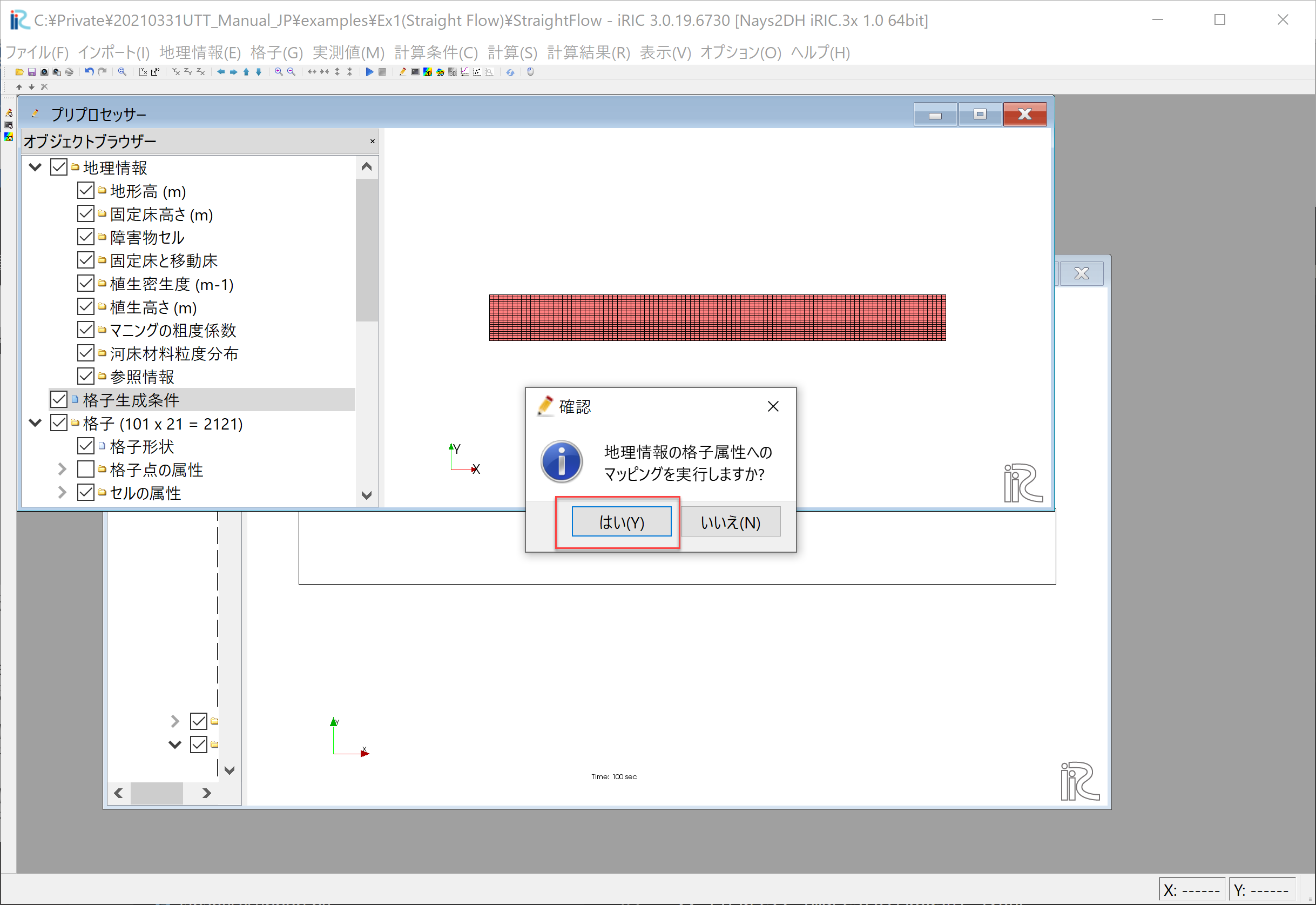
Figure 13 :確認(マッピング)
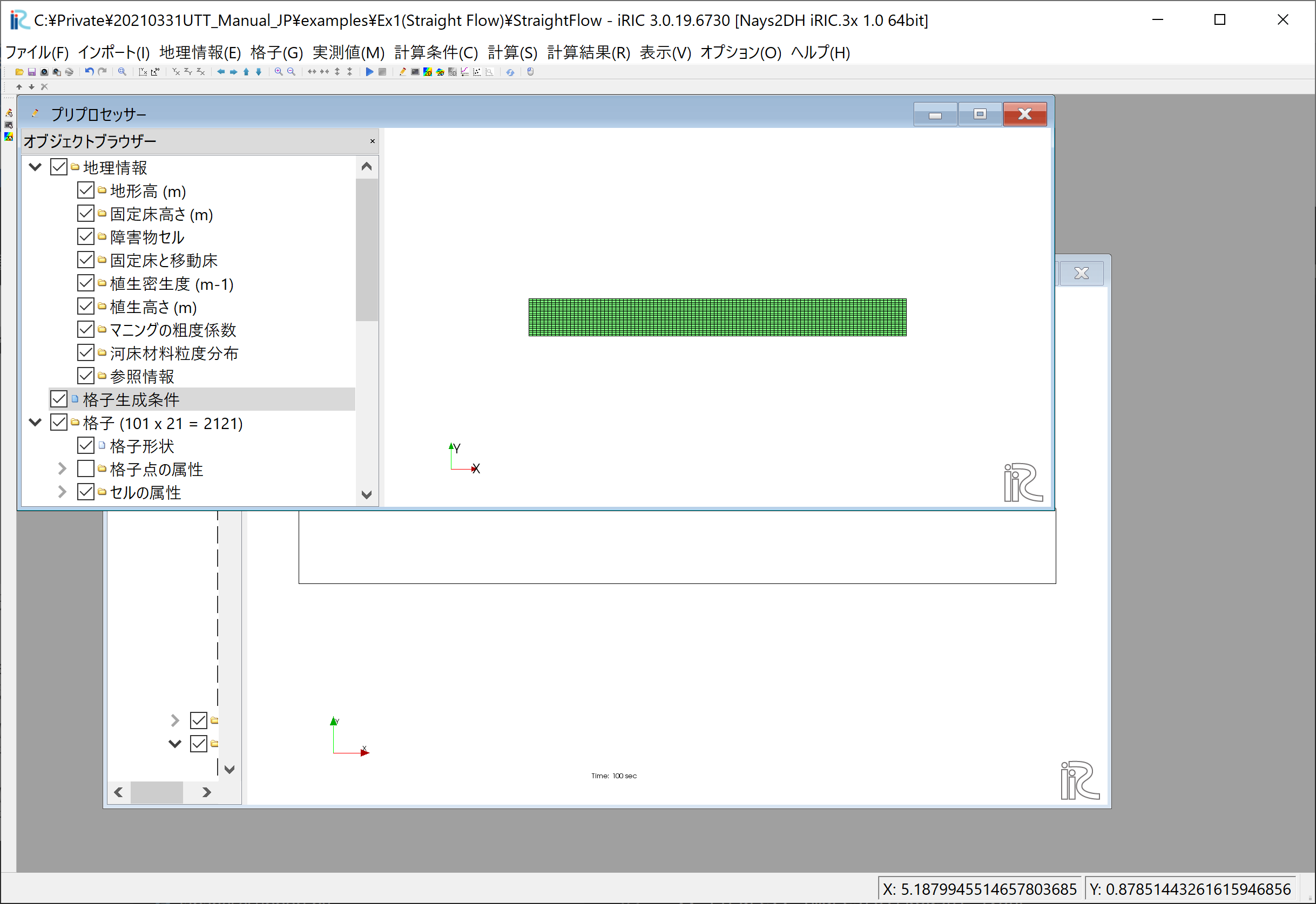
Figure 14 :格子生成完了
Nays2dHによる流れの計算条件の設定
次に計算条件の設定を行う.メニューバーから「計算条件」→「設定」を選ぶと, 計算条件設定ウィンドウ Figure 15 が表示される.
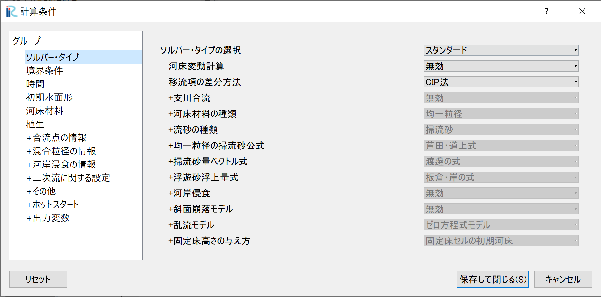
Figure 15 :計算条件
Figure 16 の「境界条件」の「上流端流量と下流端水位の時間変化」で[Edit]を クックして,流量ハイドログラフ入力ウィンドウ Figure 17 に 移る.
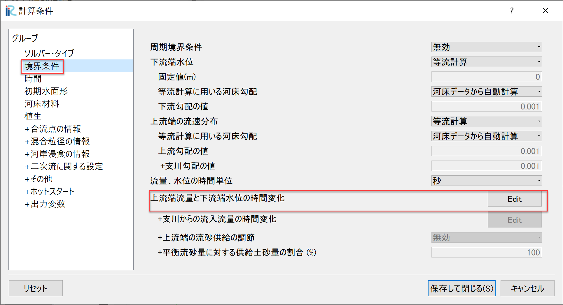
Figure 16 :流量設定
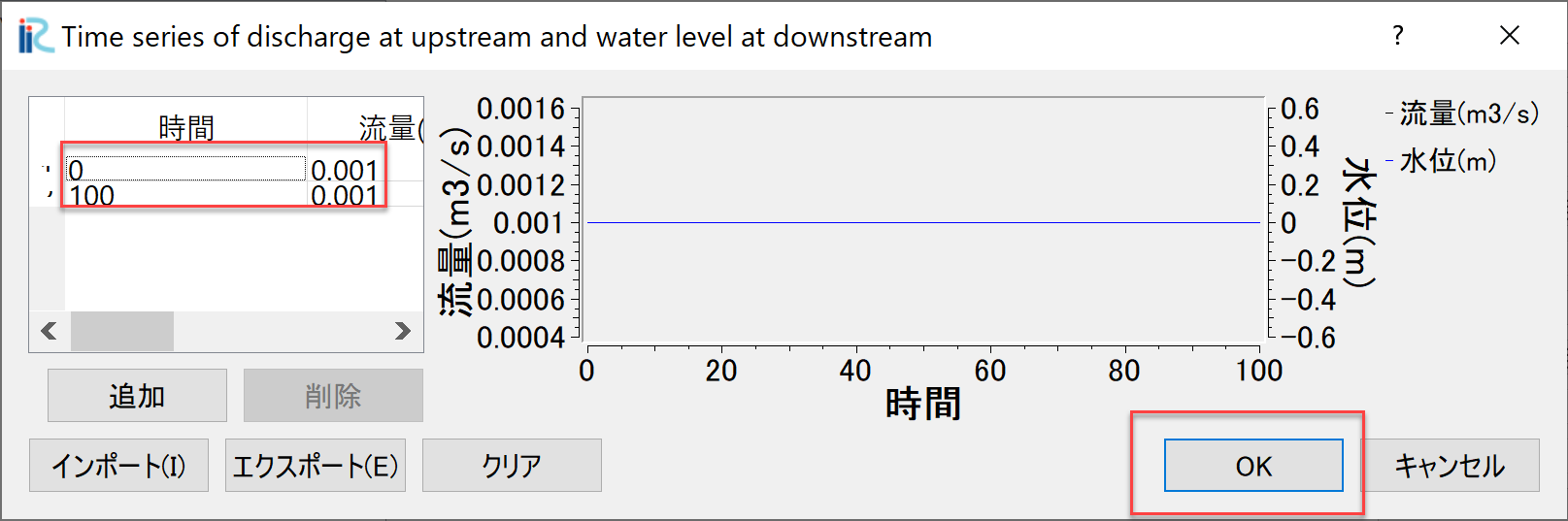
Figure 17 :流量下流端水位設定ウィンドウ
Figure 17 において,「時間」「流量」のハイドログラフを入力する. ここでは,0~100秒まで,0.001㎥/sの一定流量を与える.設定が終わったら[OK]を押して ウィンドウを閉じる.
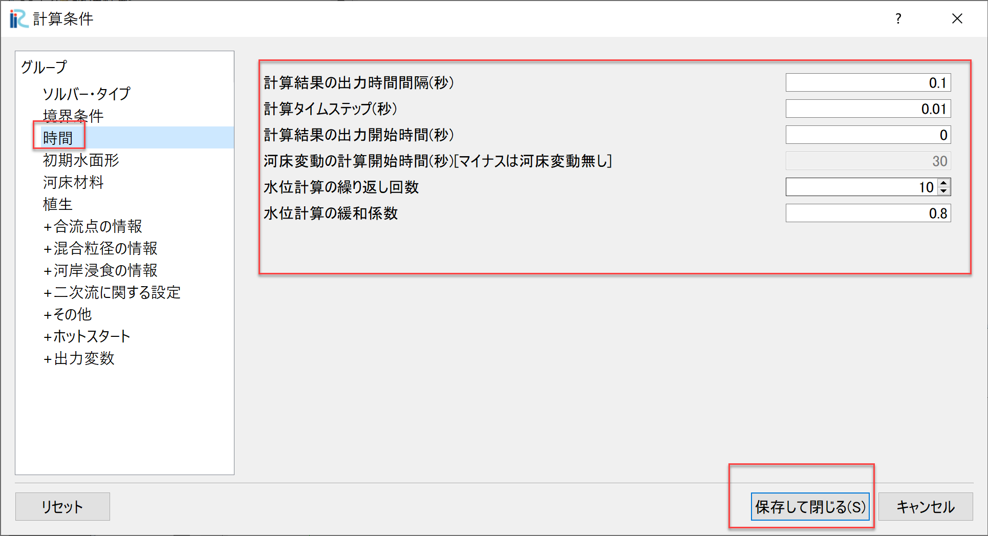
Figure 18 :時間に関するパラメータ
「時間」を選択し,パラメーターは Figure 18 のように設定し, 「保存して閉じる」をクリックする.
Nays2dHによる流れの計算実行
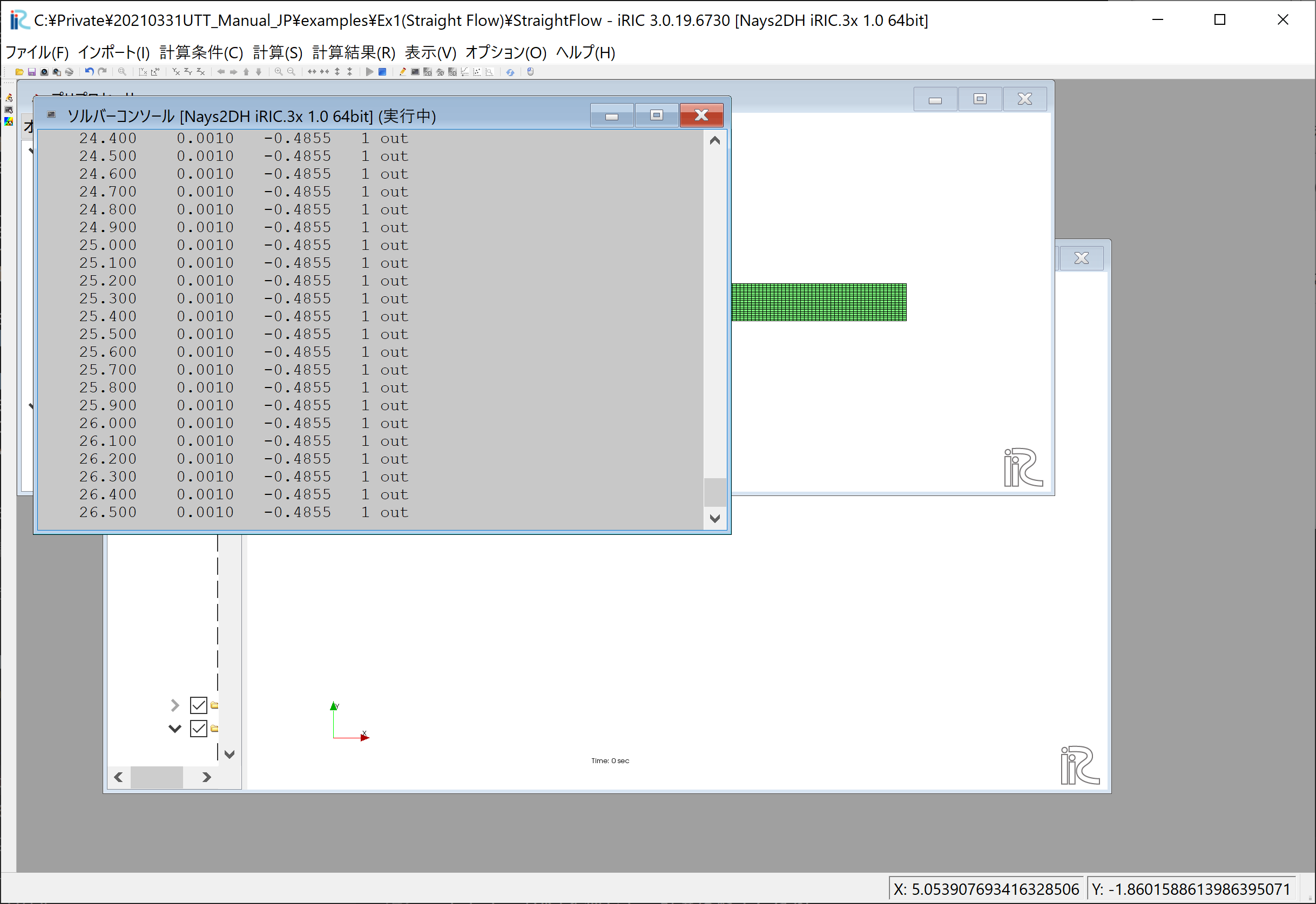
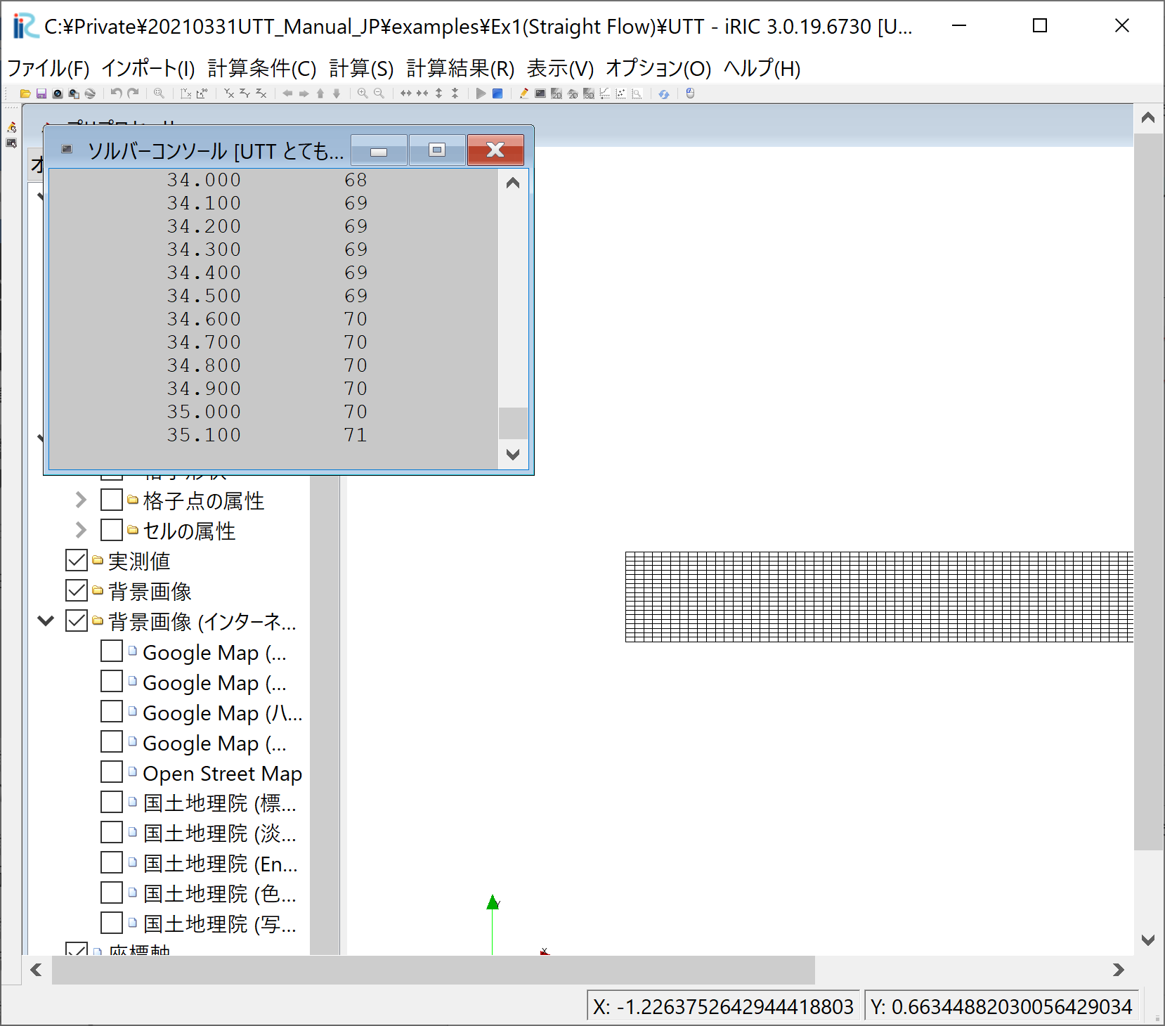
Figure 19 :計算実行中の画面
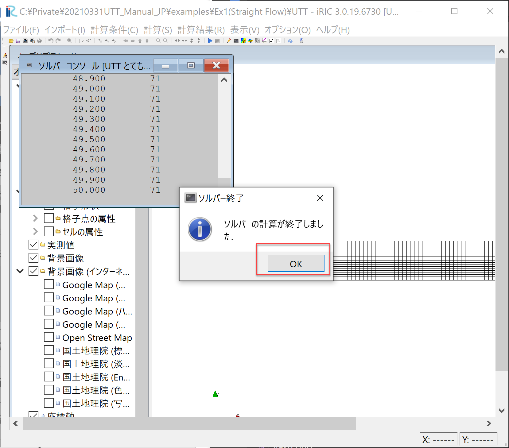
[計算]→[実行]を指定すると,「計算開始する前に,プロジェクトを保存しますか?」 など聞かれるので,「はい(Y)」を選択しプロジェクトを適当な名前で保存する. この時.プロジェクトはiproファイルで保存せずに必ずフォルダで保存すること. 計算中は Figure 19 のような画面が表示され,計算が修了すると, 終了すると,Figure 20 のような画面が現れるので, [OK]を押して,計算は終了となる.
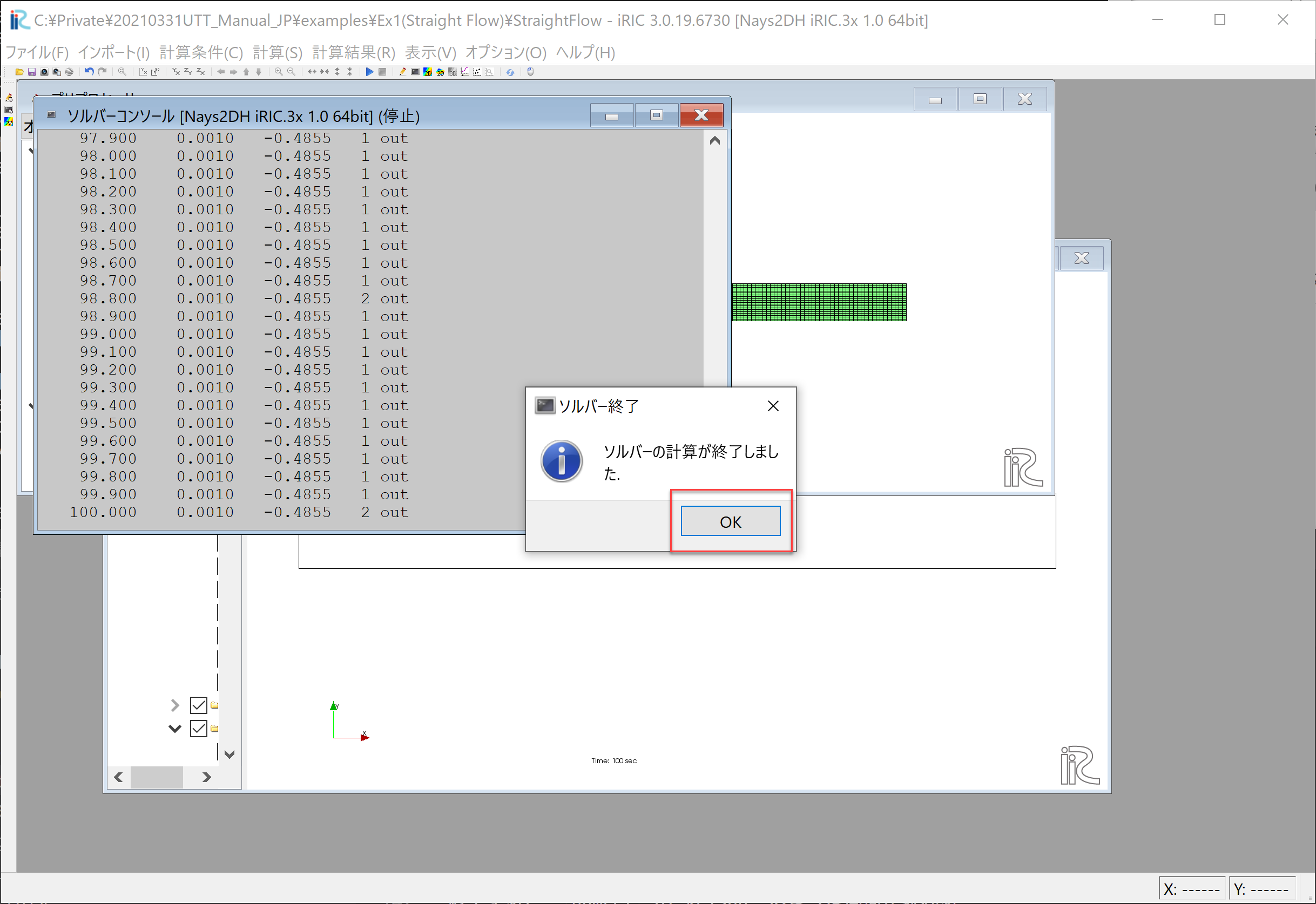
Figure 20 :計算の終了
重要 計算が終わったら必ず Figure 21 のメニューバーの「ファイル」「保存」を 選んで計算結果を保存すること.この結果は後に行うUTTによる解析で重要となる.
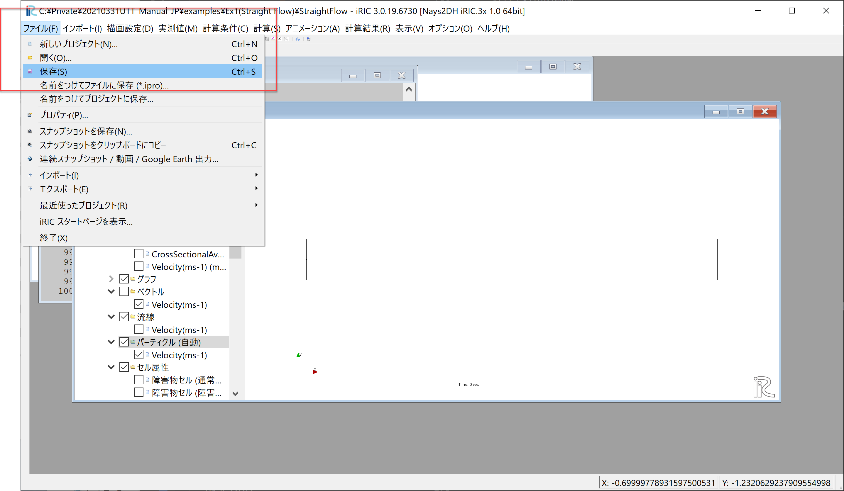
Figure 21 :計算結果の保存
計算結果の表示
計算の終了後,[計算結果]→[新しい可視化ウィンドウ(2D)を開く]を選ぶことによって,可視化ウィンドウが現れる.
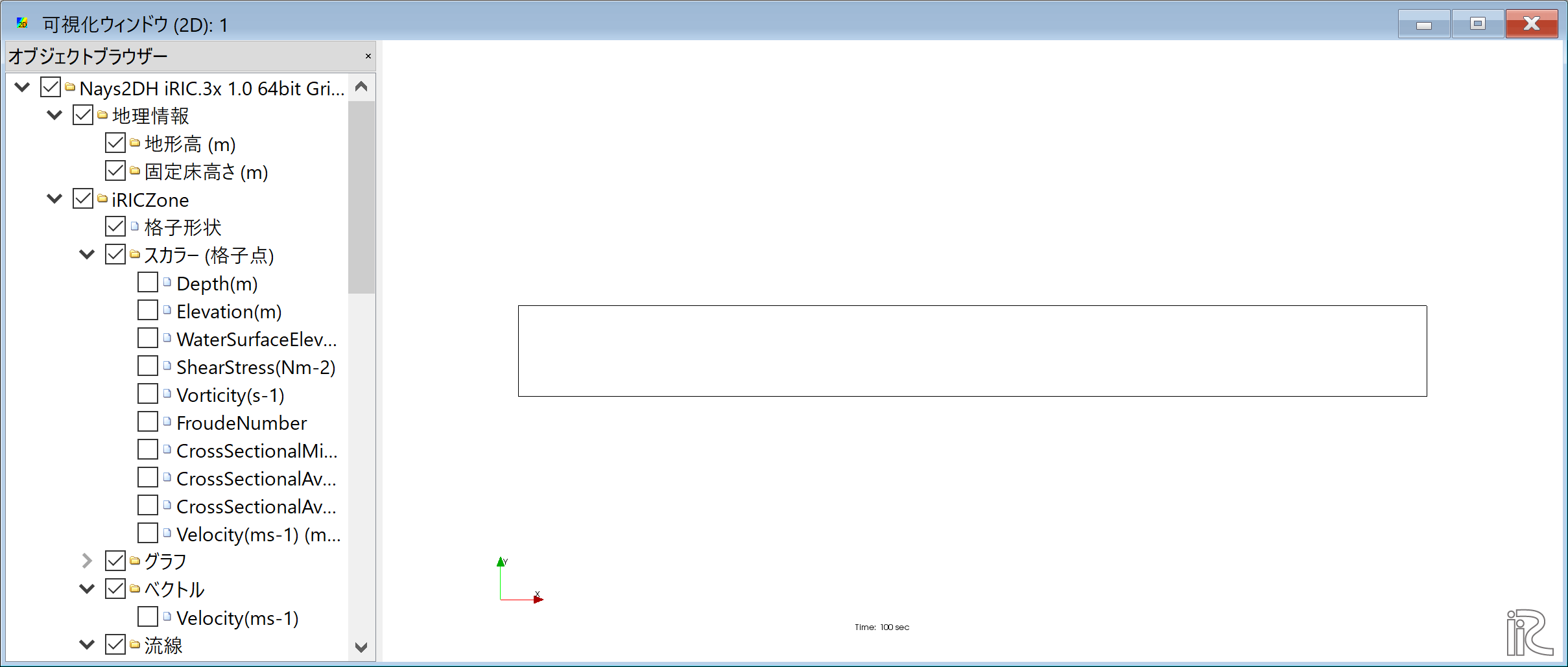
Figure 22 : 計算結果の表示
流速ベクトルの表示
オブジェクトブラウザーで,[ベクトル][Velocity]に☑マーク入れて, [ベクトル]をフォーカスさせてマウス右ボタン[プロパティ]をクリックすると, 「ベクトル設定」ウィンドウ Figure 23 が現れる.ここで,赤線で 囲った部分の設定をして[OK]を 押すと Figure 24 が表示される. Figure 24 は水深平均流速ベクトル である.等流状態で一様の流速分布となっている.
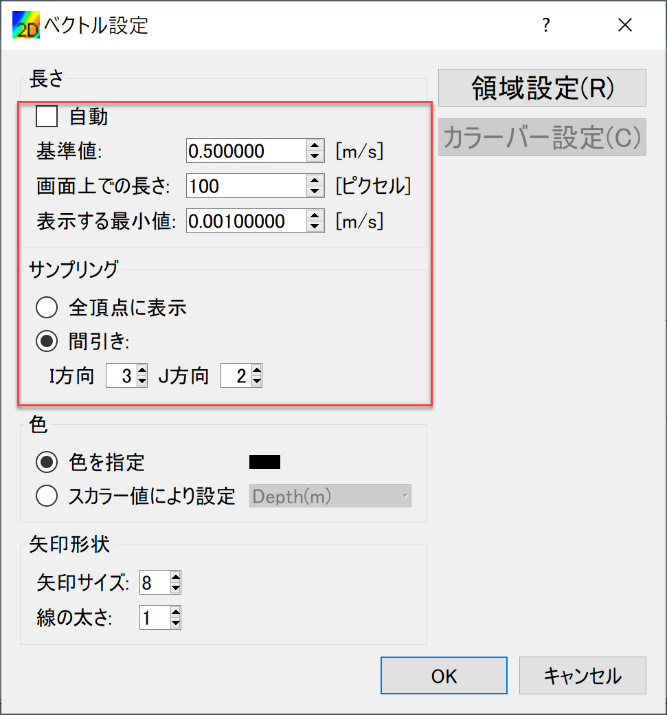
Figure 23 : ベクトル設定
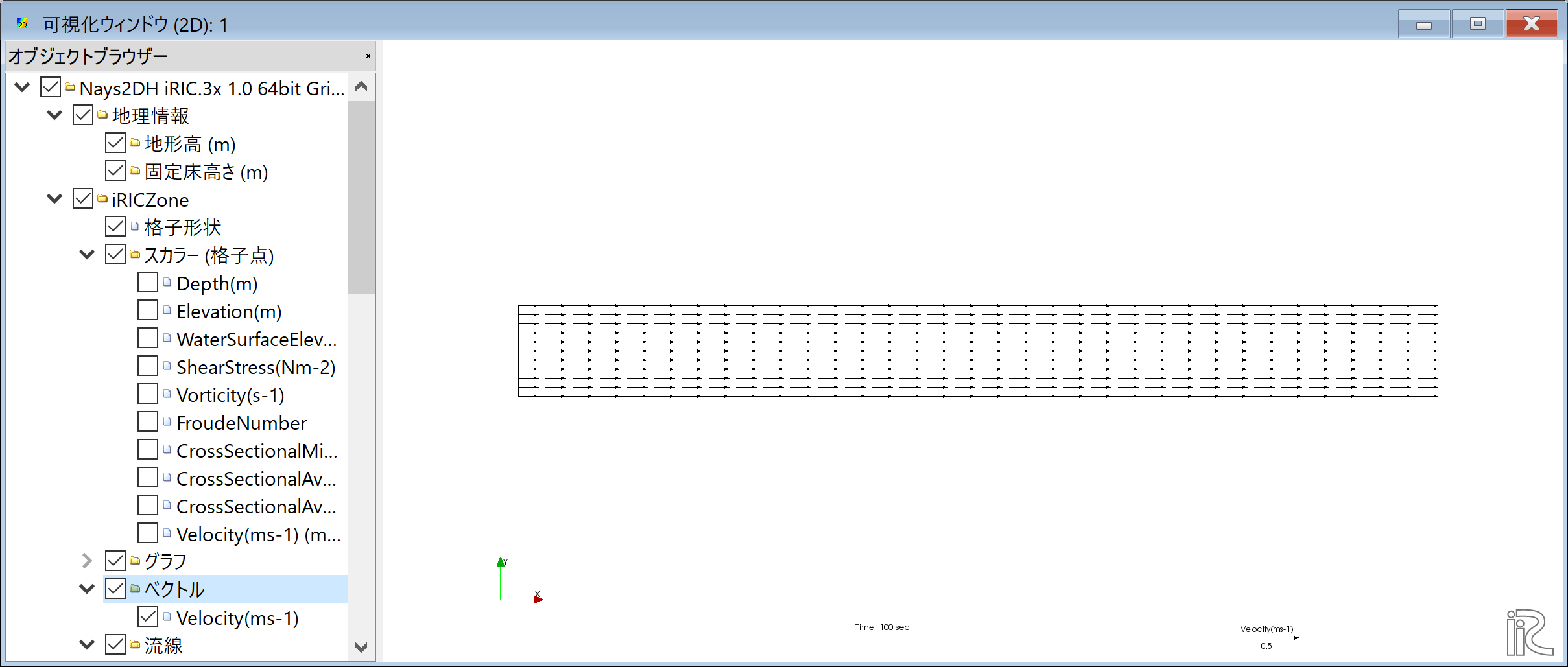
Figure 24 : 水深平均流速ベクトル表示
パーティクルの表示
オブジェクトブラウザーの「ベクトル」を一旦アンチェックし,「パーティクル」と「Velocity」 に☑マークを入れる.( Figure 25 )
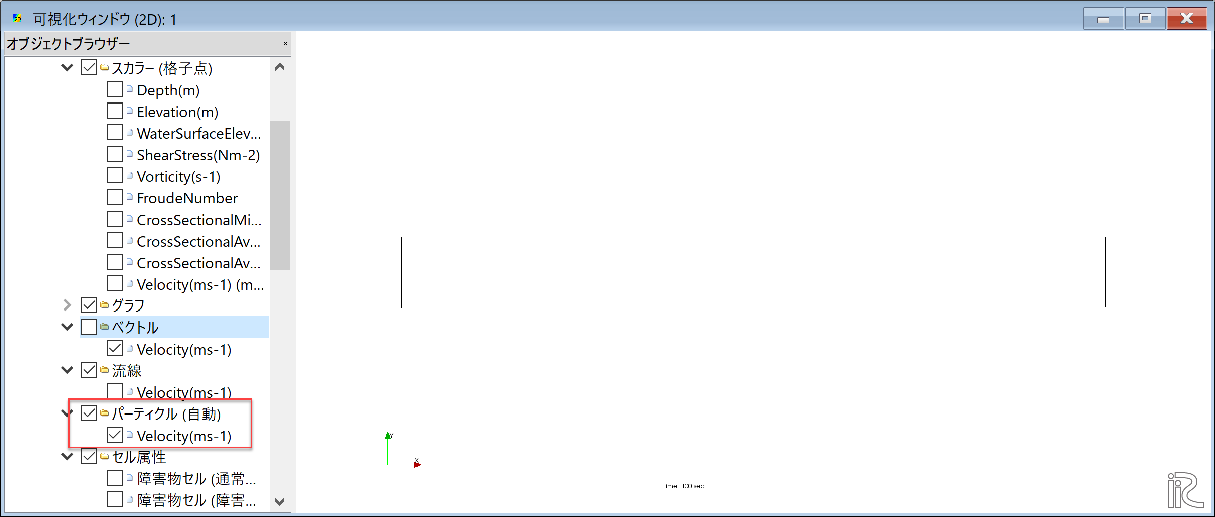
Figure 25 : パーティクル(1)
Figure 26 のように「パーティクル」右クリックして「プロパティ」を選ぶと,
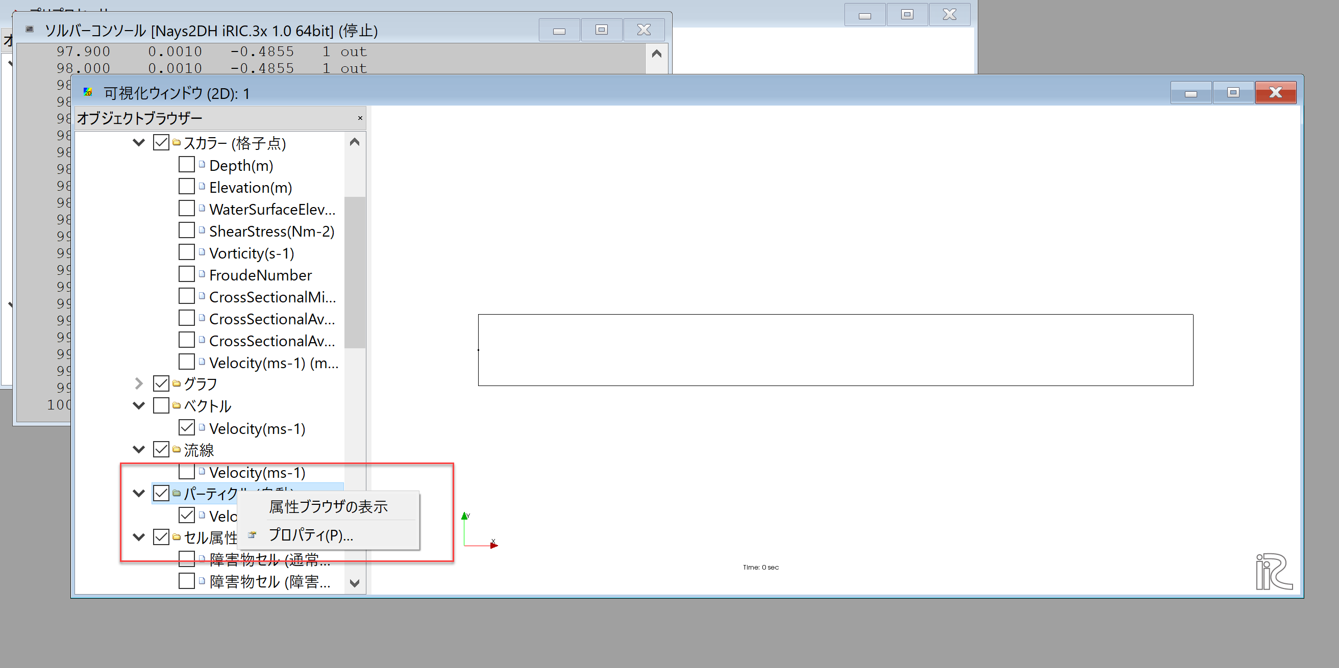
Figure 26 : パーティクル(2)
Figure 27 のような「パーティクルの設定」画面が現れるので,図の赤囲いのように パーティクスの発生位置を指定する.
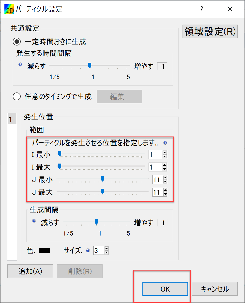
Figure 27 : パーティクルの設定
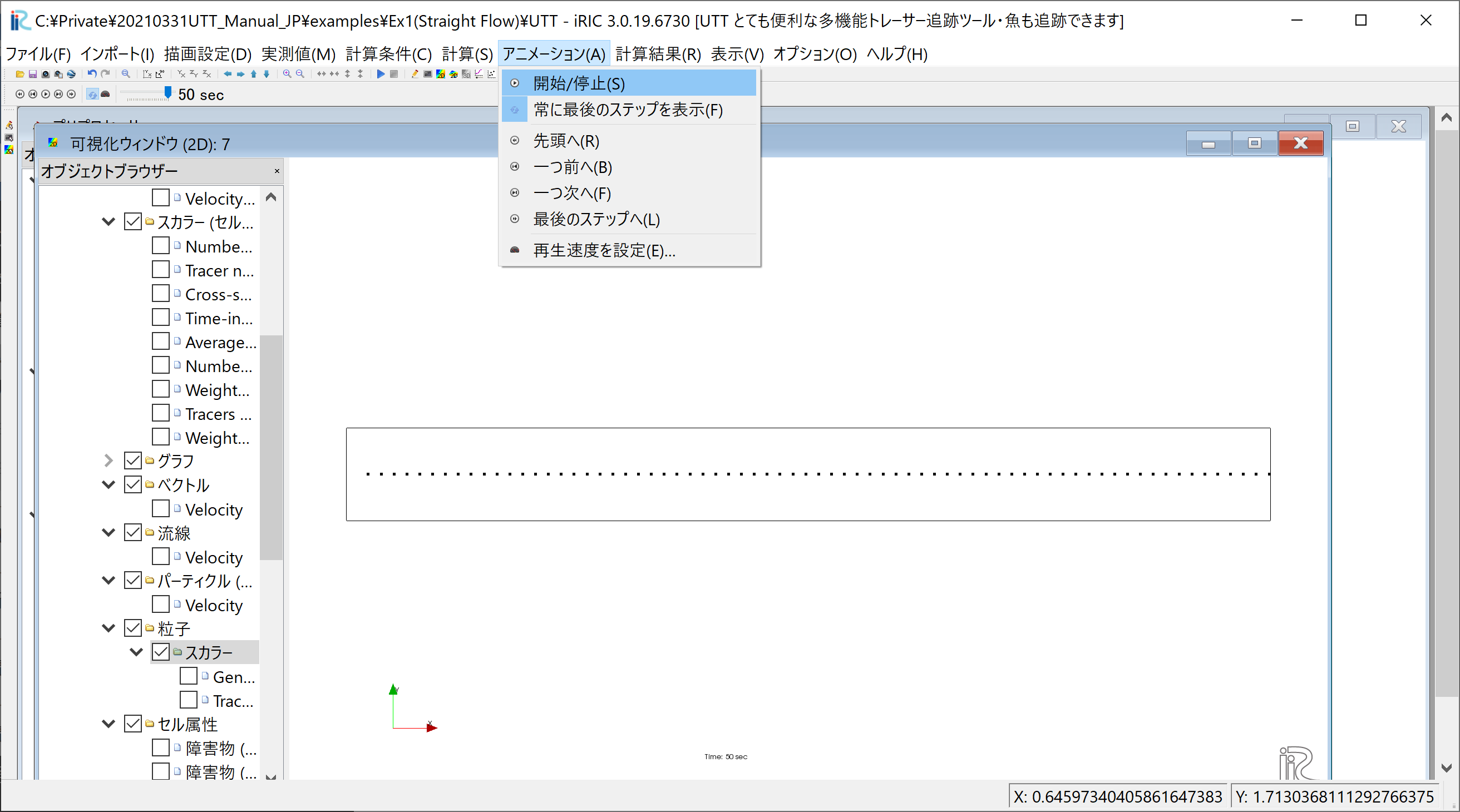
Figure 27 に示すように,タームバーをゼロに戻し,メインメニューから, 「アニメーション」「開始/停止」を選ぶことにより, Figure 29 のようなパーティクルの動きが表示される.
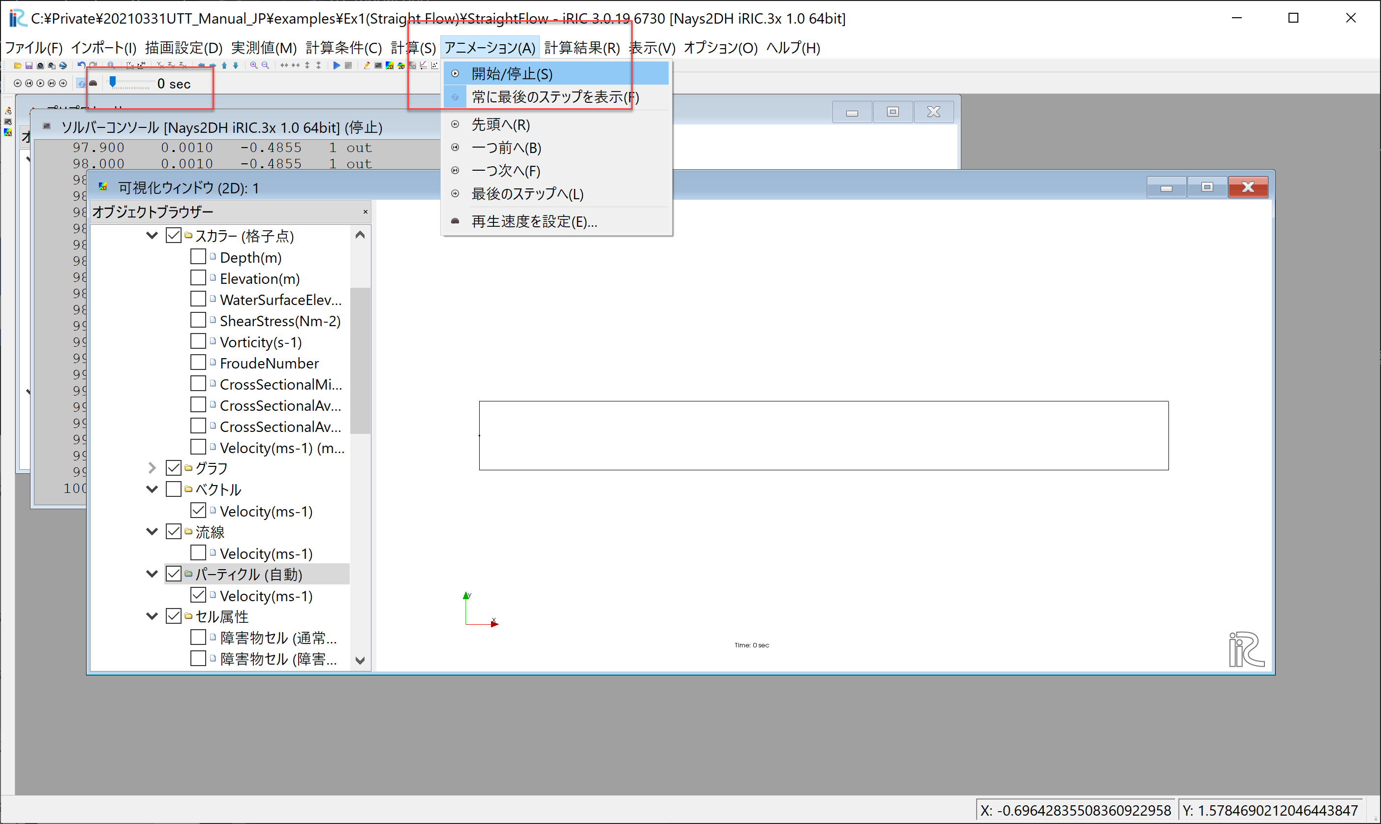
Figure 28 : アニメーションの再生
Figure 29 : Nays2dhによるパーティクルアニメーション
Figure 29 からわかるよに,流れの計算結果をそのままパーティクル表示すると, 乱流による乱れ成分が含まれていないので,何の変哲も無い 単純で退屈な 表示しかされない( ^^) _U~~
UTTよるトレーサーの追跡
UTTの起動
iRICの起動画面から,[新しいプロジェクト]を選ぶと表示されるソルバの選択画面で, 「UTTとても便利な多機能トレーサー追跡ツール・魚も追跡できます」を選んで,「OK」を クリックする.( Figure 30 )
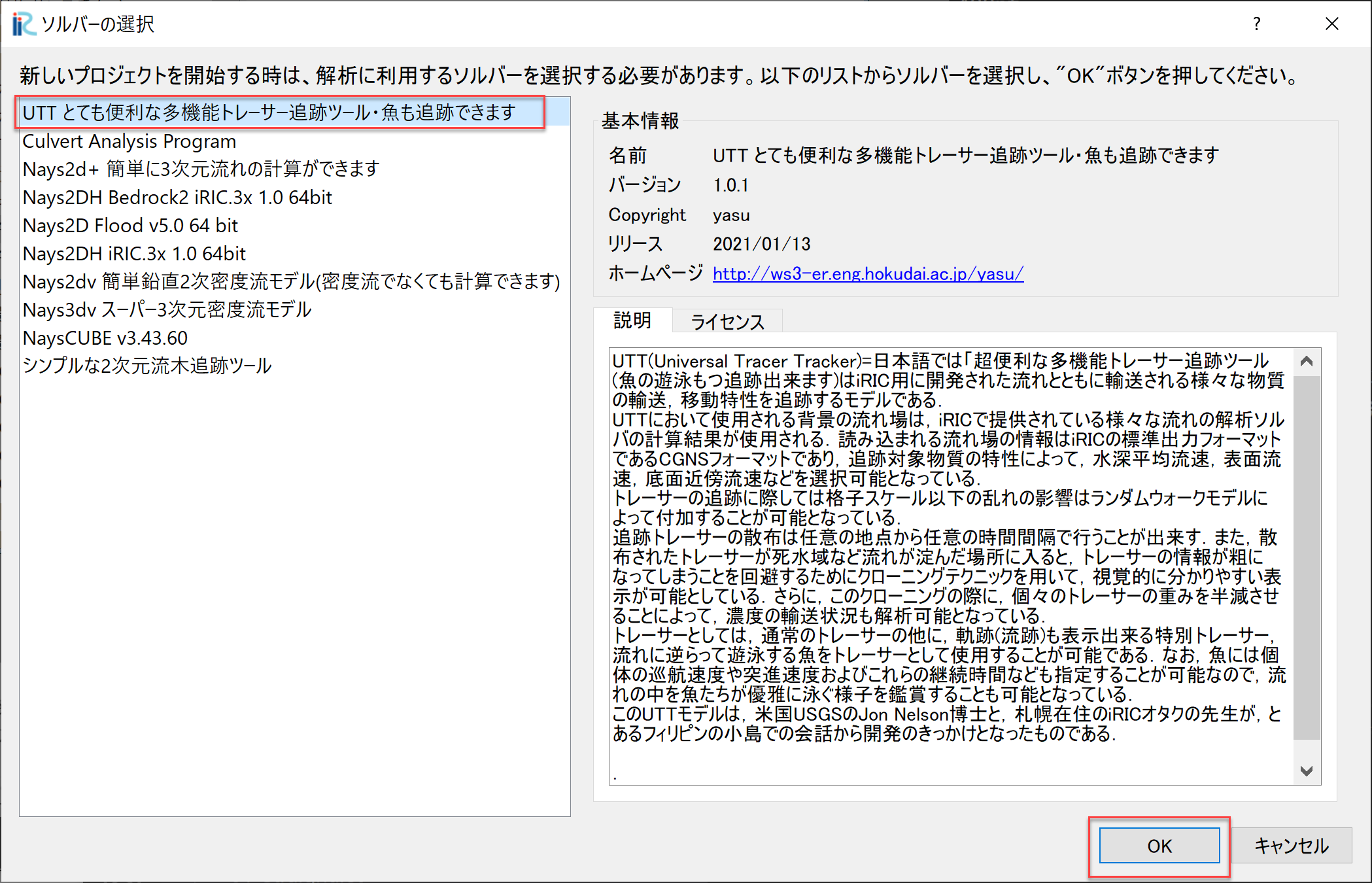
Figure 30 : UTTの選択と起動
「無題 -iRIC 3.0.xxxxx [UTTとても便利な多機能トレーサー追跡ツール・魚も追跡できます]」 と書かれたウインドウが現れ,UTTセッションが開始される.(Figure 31 )
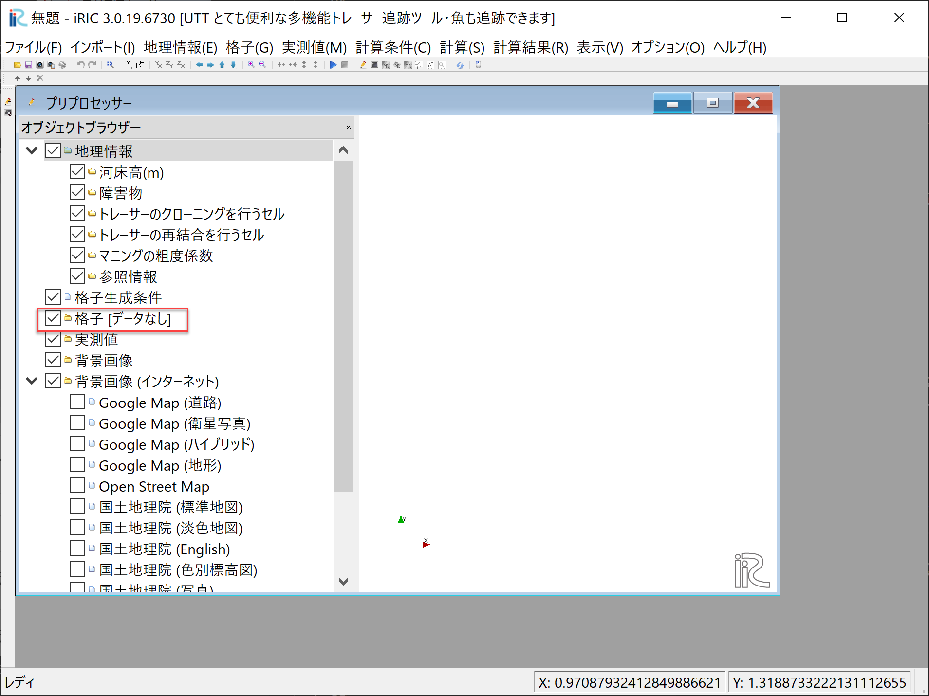
Figure 31 : UTTの起動
この状態の「プリプロセッサー」の「オブジェクトブラウザー」の「格子」の部分には [データなし]と表示されている( Figure 31 ) ので,まずは前記 01_lavel_koshi で作成したものをインポートする.
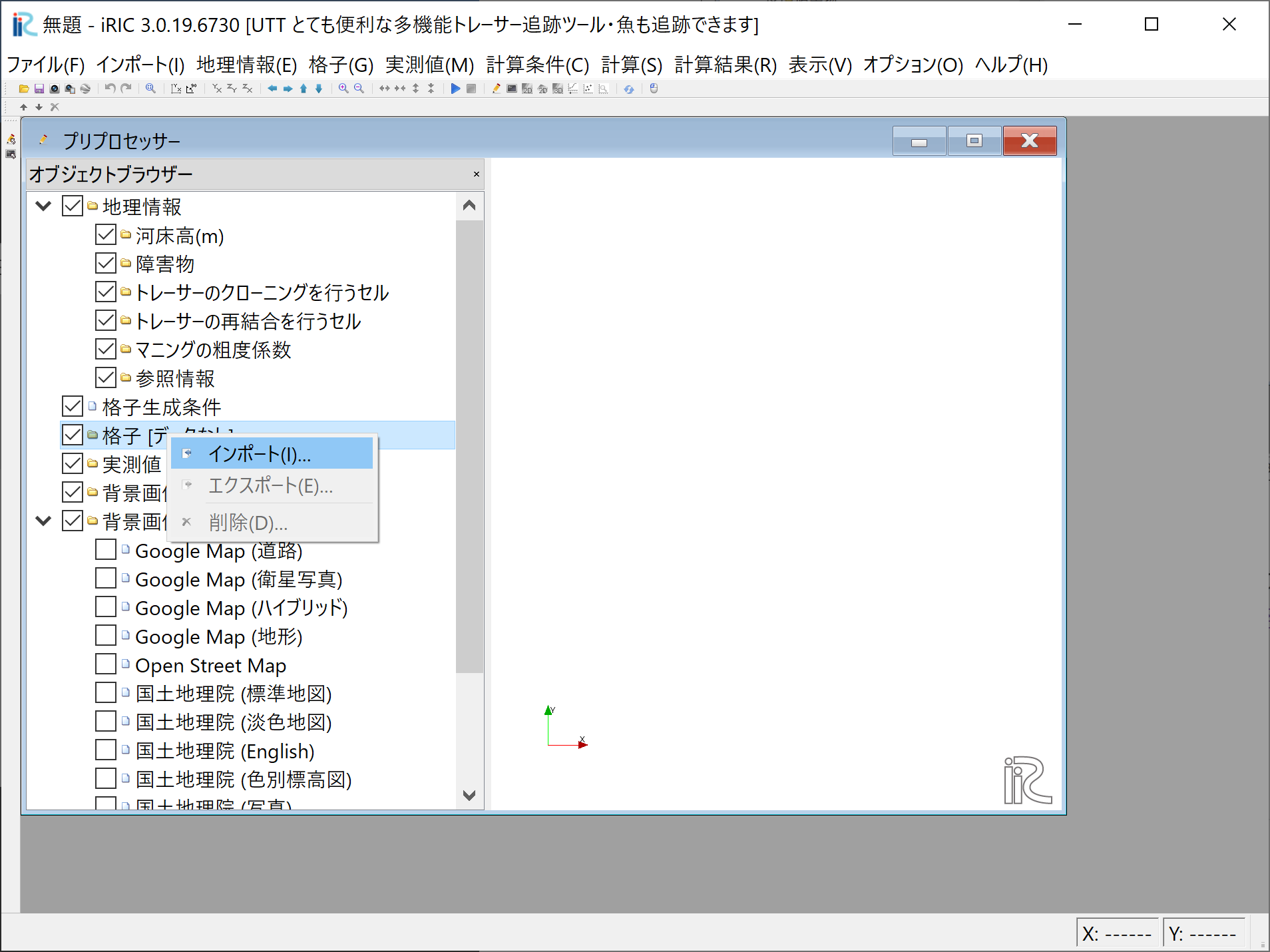
Figure 32 : 格子データのインポート
「格子(データーなし)」を右クリックして「インポート」を選ぶ (Figure 32 ).

Figure 33 : 格子データファイルの選択
Figure 33 に示すように前述の「Nays2DHによる計算結果」を セーブしたプロジェクトフォルダーの中にある 「Case1.cgn」を選択して,「開く」をクリックする.
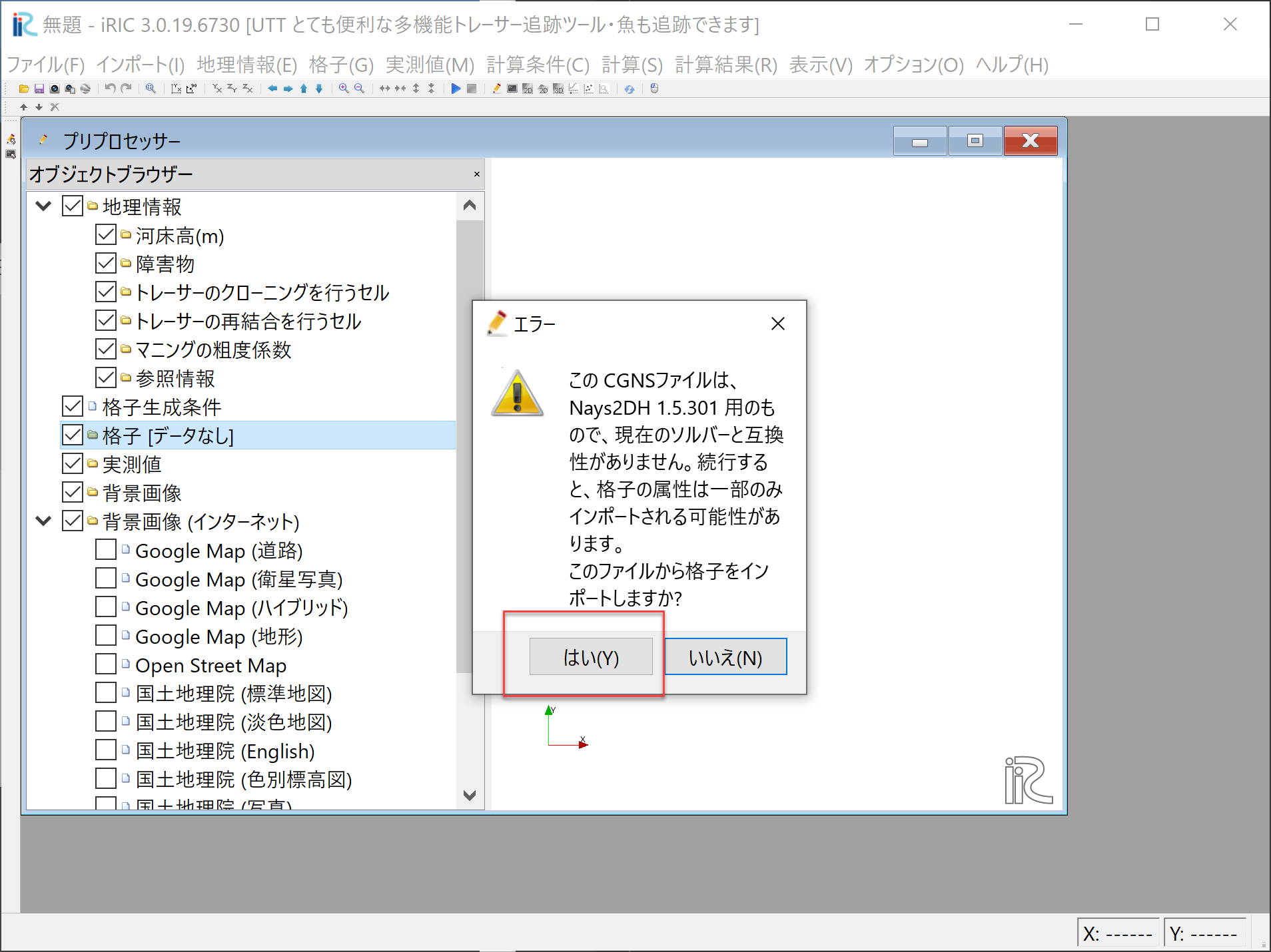
Figure 34 : 警告
Figure 34 「このCGNSファイルは・・・ナンチャラ・・・・インポートしますか?」 と出るが,細かいことは気にせずに「はい(Y)」と答えると, Figure 35 のように格子のインポートが完了する.
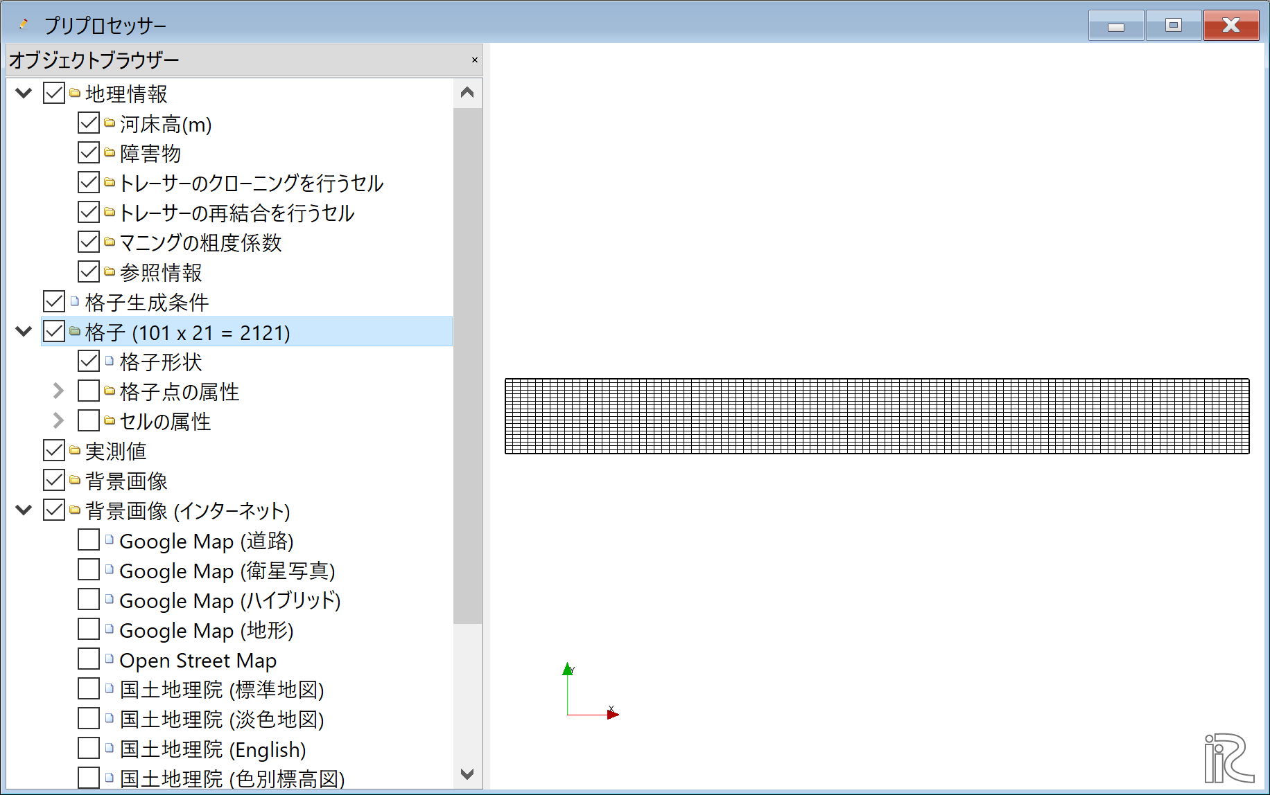
Figure 35 : 格子のインポート完了
1個のトレーサーの追跡(乱流拡散無し)
計算条件の設定
Figure 36 に示すように,メインメニューから「計算条件」「設定」を選ぶ.
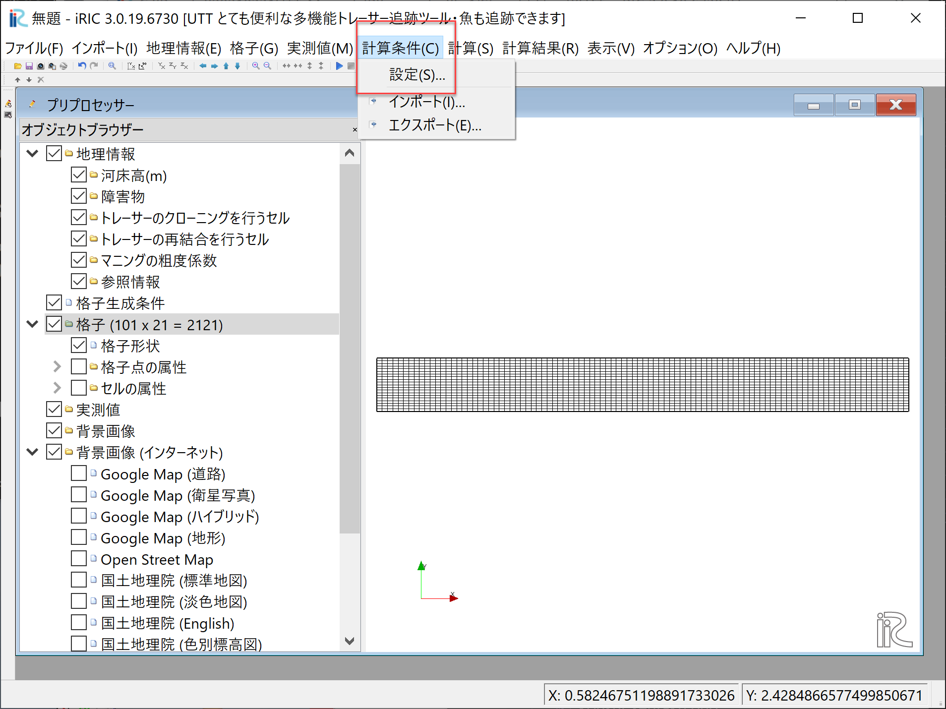
Figure 36 : 計算条件の設定(0)
Figure 37 に示すように,「基本設定」 「流れの計算結果を読み込むCGNSファイル」を指定する.通常は,前記の「Nays2DHの計算結果」 が格納されているCGNSファイルを指定する.
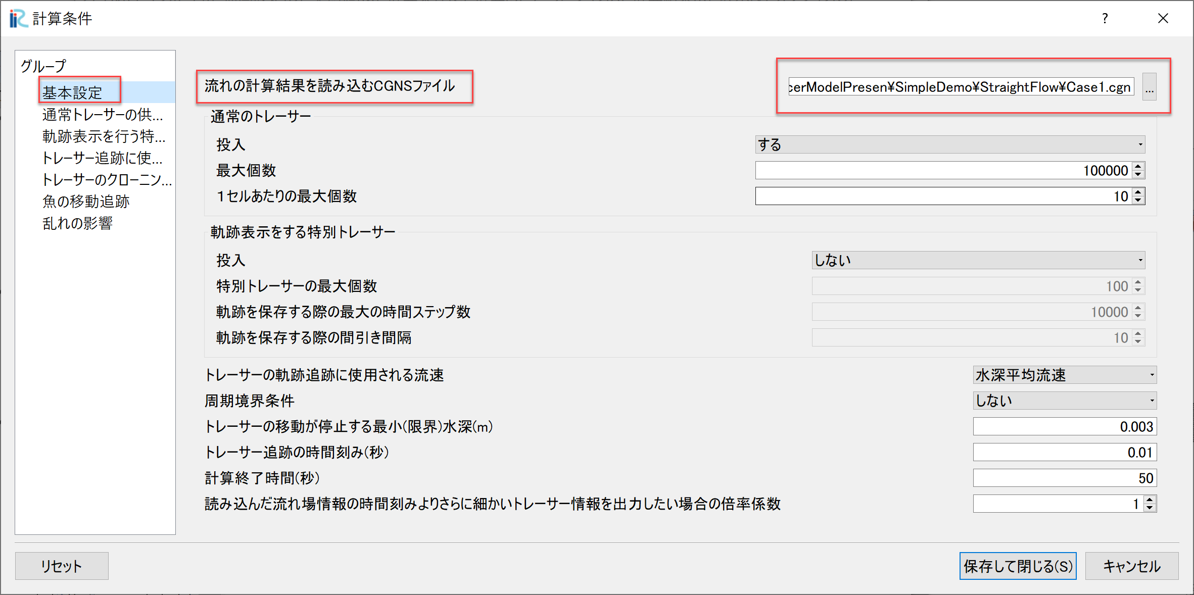
Figure 37 : 計算条件の設定(1)
. _01_utt_joken_2:
「基本設定」の上記以外の部分は,Figure 38 に示すように 設定する.なお.使用するトレーサーは「通常のトレーサー」のみで 「特別トレーサー」は使用しない.
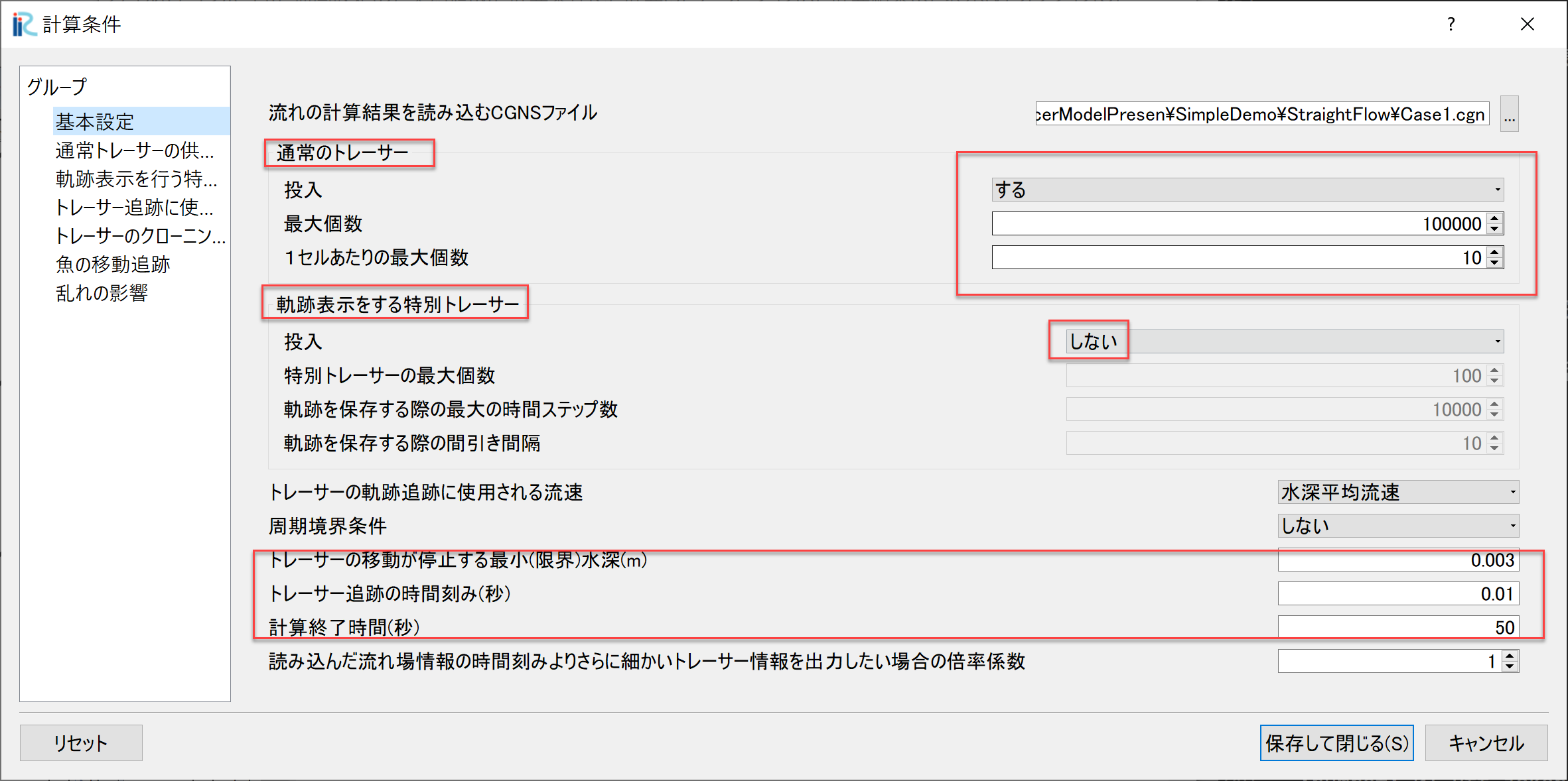
Figure 38 : 計算条件の設定(2)
「通常トレーサーの供給条件」は,UTTにおけるトレーサーの位置情報の記述方法 で述べた表示方法に したがって,Figure 39 のように設定する.
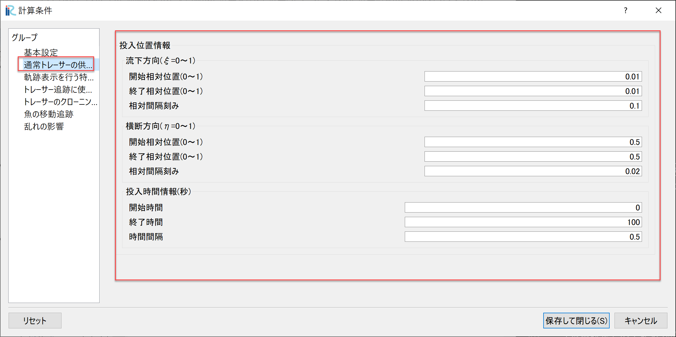
Figure 39 : 計算条件の設定(3)
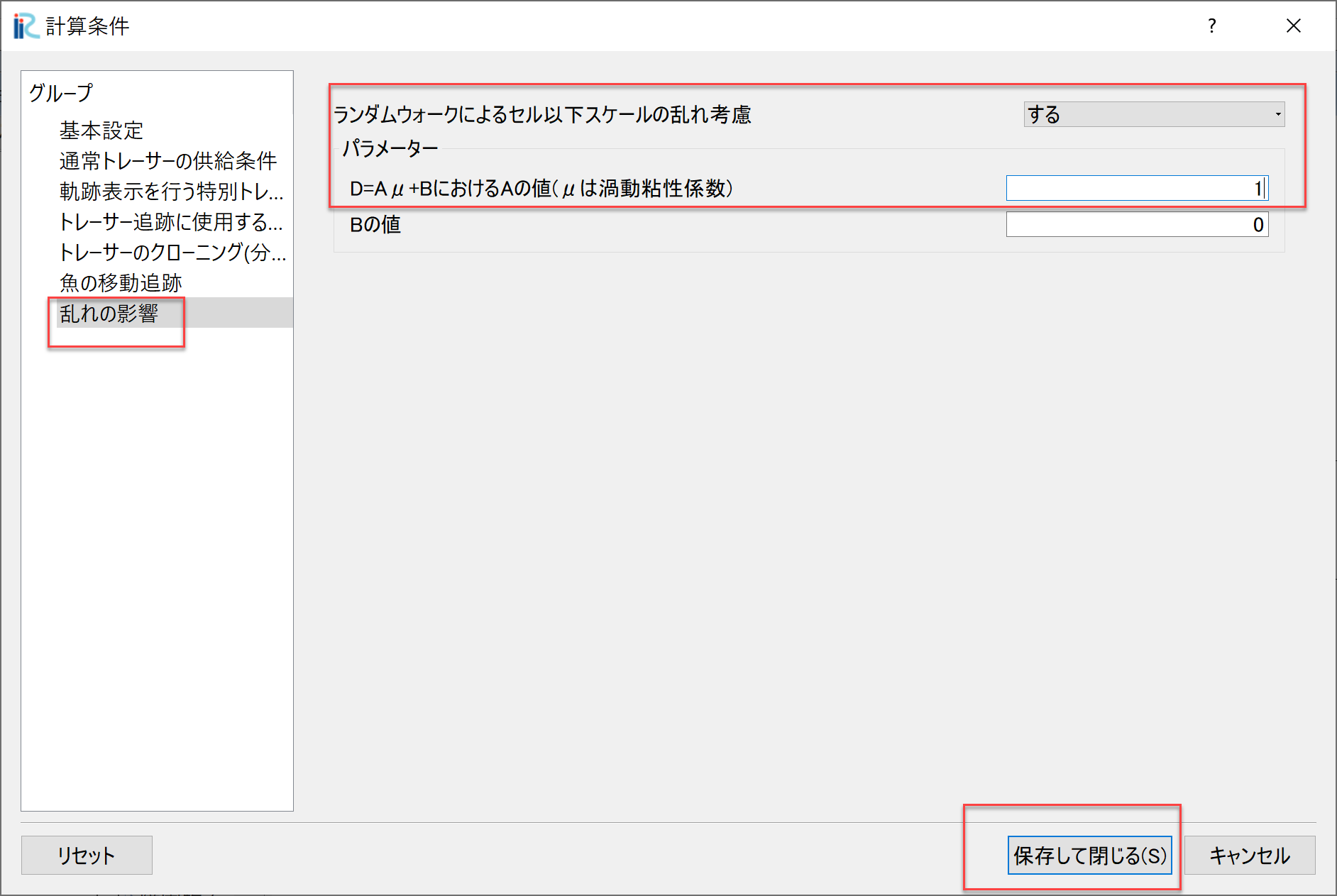
「乱れの影響」の「ランダムウォークによるセル以下スケールの乱れの考慮」 は Figure 40 に示すように「しない」に設定して, 「保存して閉じる」を選択する.
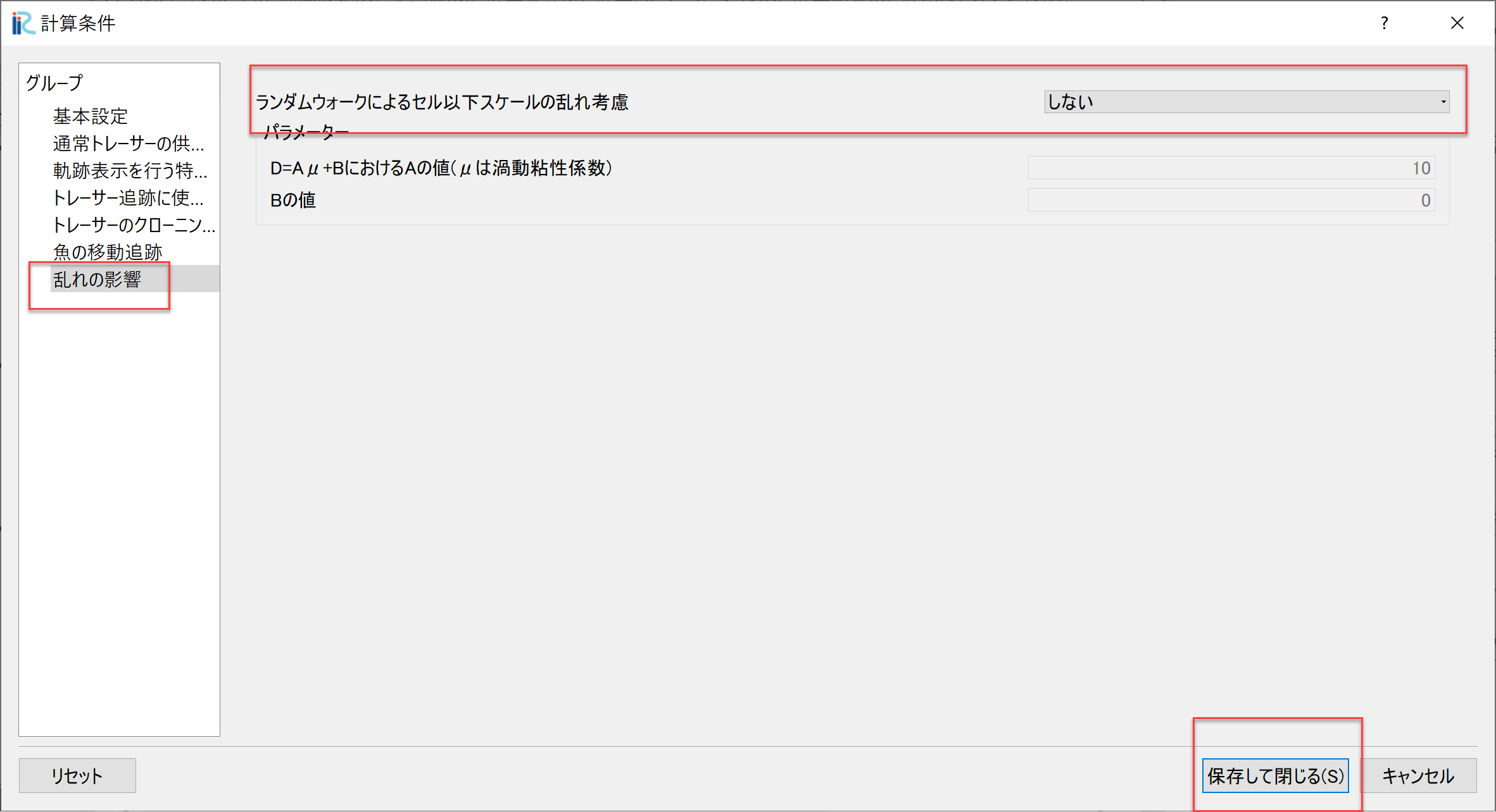
Figure 40 : 計算条件の設定(4)