[計算例 1]60°単純曲線水路
Nays2d+で簡単な湾曲水路の準3次元計算をします.
ソルバの選択
iRICの起動画面から,[新しいプロジェクト]を選ぶと表示されるソルバの選択画面で, [Nays2d+ 簡単に3次元流れの計算ができます]を選んで[OK]ボタン押すと,
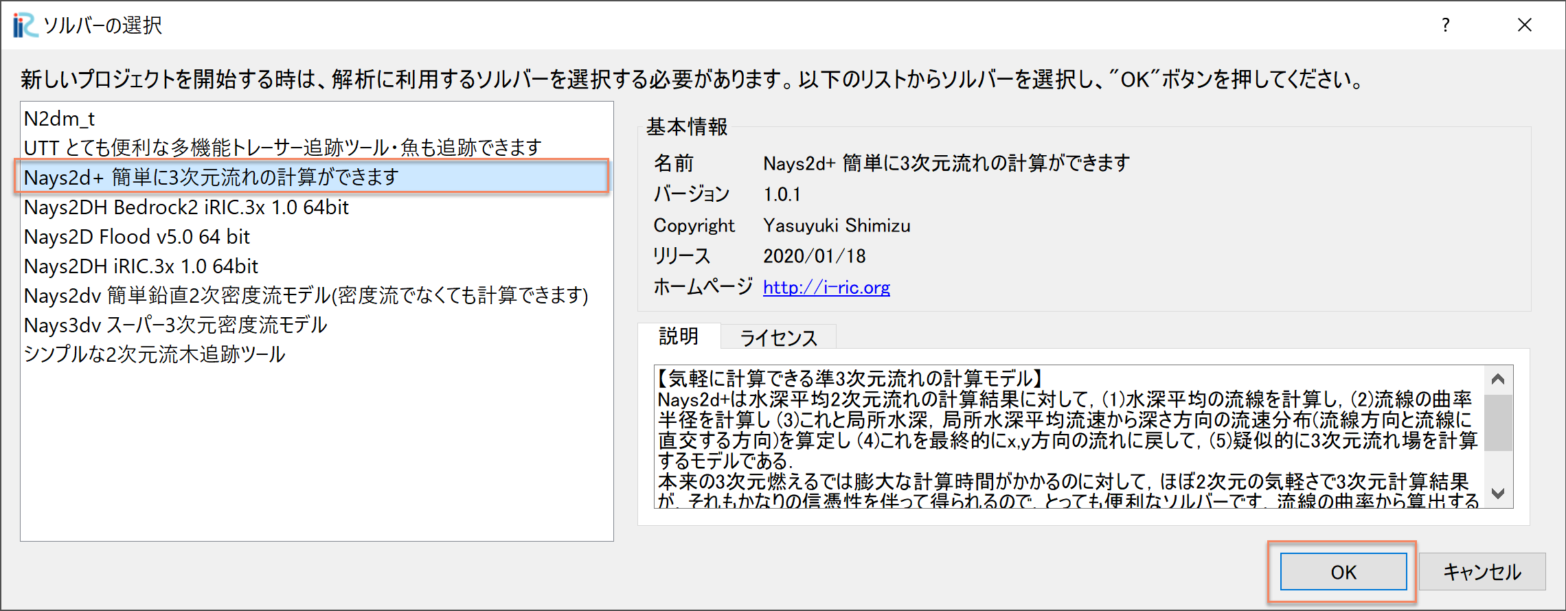
Figure 4 : ソルバーの選択
「無題- iRIC 3.x.xxxx [Nays2d+ 簡単に3次元流れの計算ができます]」と書かれた Windowが現れる.
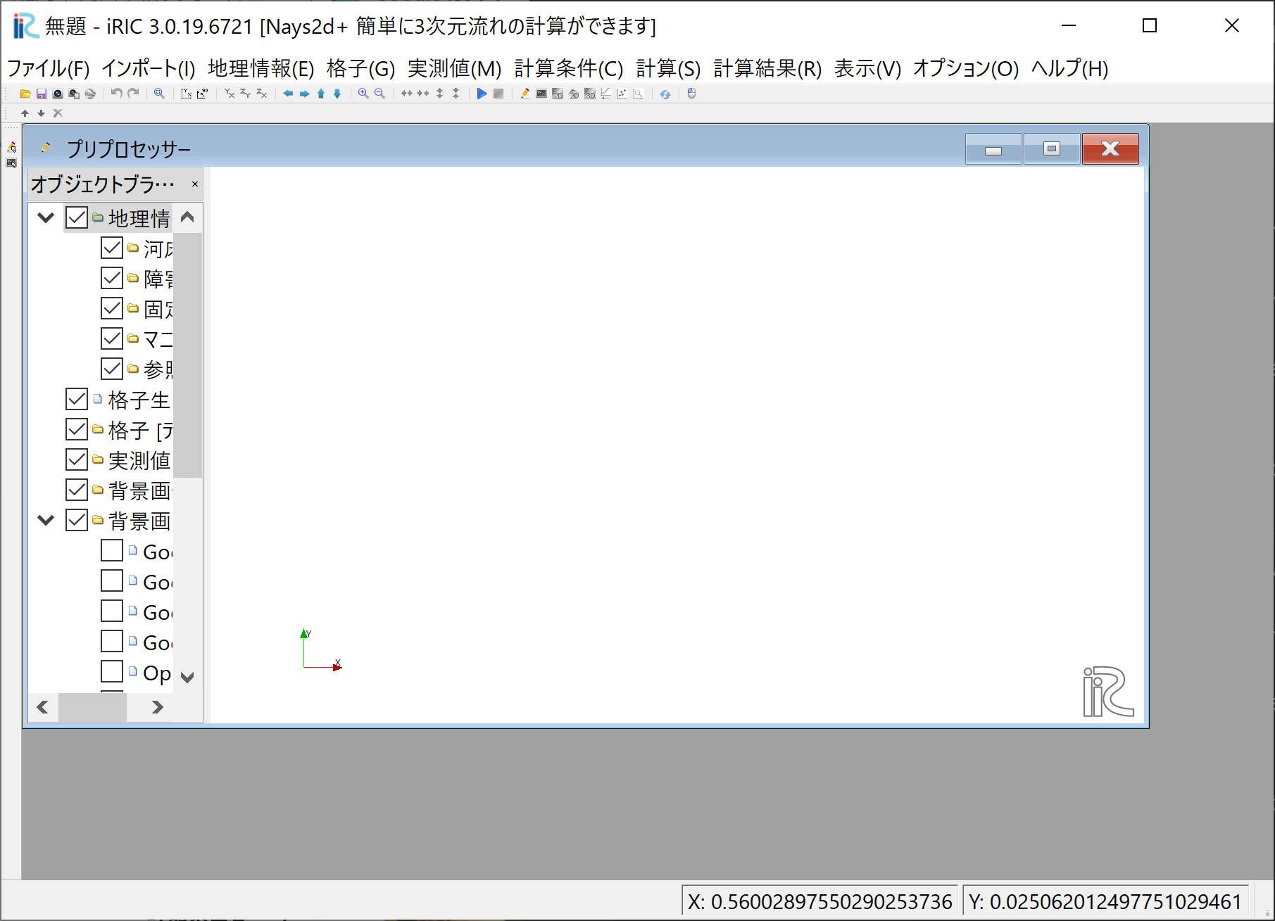
Figure 5 : 無題
Figure 5 のウィンドウで,[格子]→[格子生成アルゴリズムの選択]から現れる, 「格子生成アルゴリズムの選択」ウィンドウ で[2次元円弧形水路格子生成ツール]を選んで[OK]を押す.
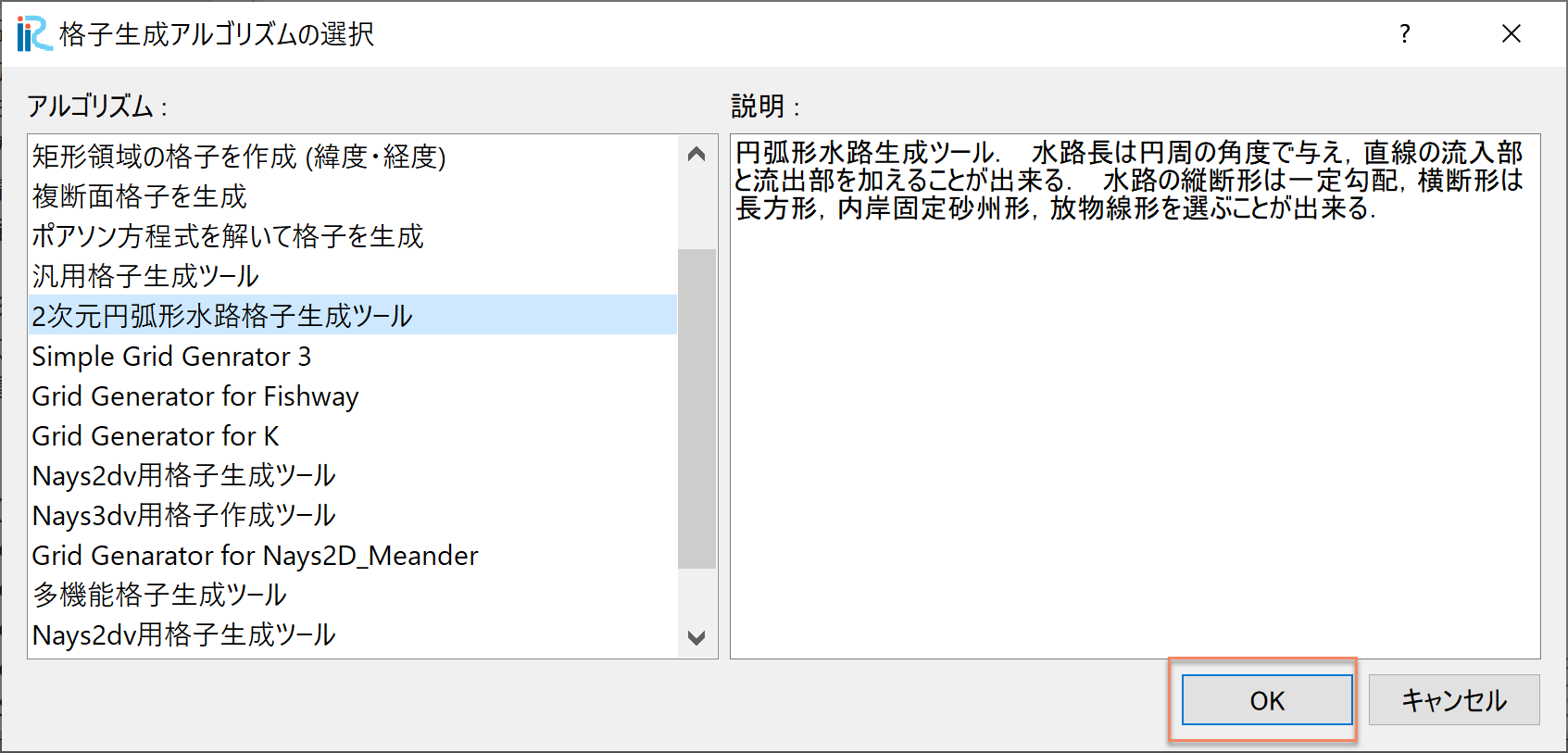
Figure 6 : 格子生成アルゴリズムの選択
計算格子の作成
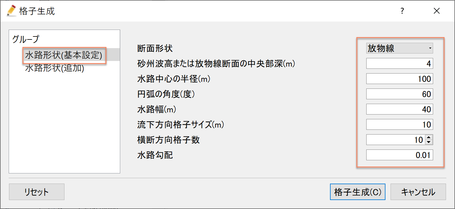
Figure 7 :水路形状(基本設定)
Figure 7 の画面で,「水路形状(基本形状)」を選択し, 「断面形状」を[放物線],「砂州波高または放物線断面の中央部深(m)」を[4], 「水路中心の半径(m)」を[4],「円弧の角度(度)」を[60],「水路幅(m)」を[40], 「流下方向格子サイズ(m)」を[10],「横断方向格子数」を[10],「水路勾配」を[0.01]に 設定する.
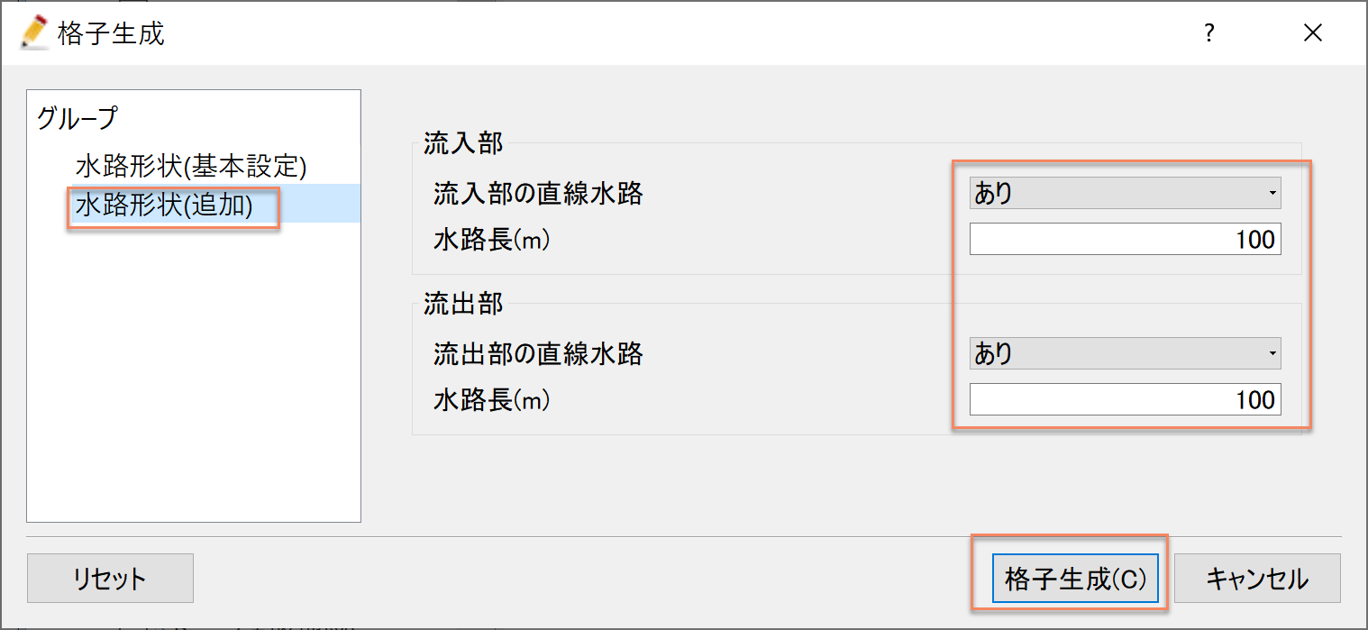
Figure 8 :水路形状(追加)設定
Figure 8 の画面で,「流入部」「流出部」をいずれも[あり],「長さ」を[10]mに 設定し,最後に[格子生成]ボタンを押す.
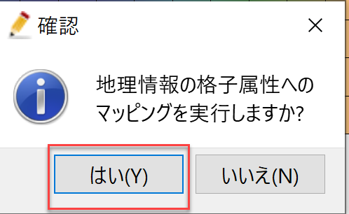
Figure 9 :確認(マッピング)
すると,Figure 9 確認ウィンドウが現れるので,[はい(Y)]を押すと格子が生成され, 下図 Figure 10 が表示される.
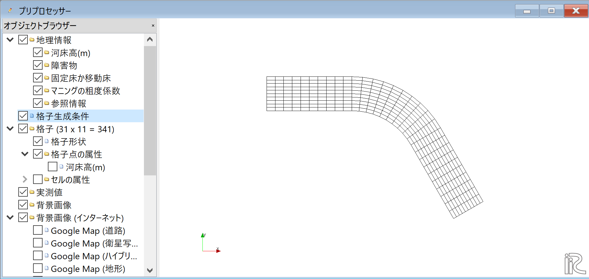
Figure 10 :格子生成完了
ここで確認のためににオブジェクトブラウザーで「格子」「格子の属性」「河床高」にチックマークを付けて 表示させると Figure 11 のように断面形が放物線形で上下流に直線部を伴う単純な曲線 水路が生成されたことが分かる.
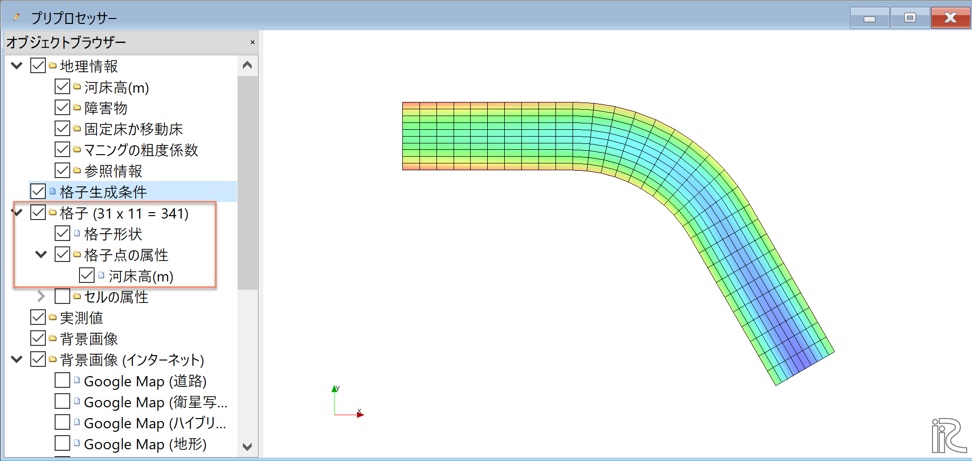
Figure 11 :格子生成完了
計算条件の設定
次に計算条件の設定を行う.メニューバーから「計算条件」→「設定」を選ぶと, 計算条件設定ウィンドウ Figure 12 が表示される.

Figure 12 :モデルパラメータ
Figure 13 の「流量および読み込みファイル」で[Edit]を クックして,流量ハイドログラフ入力ウィンドウ Figure 14 に 移る.
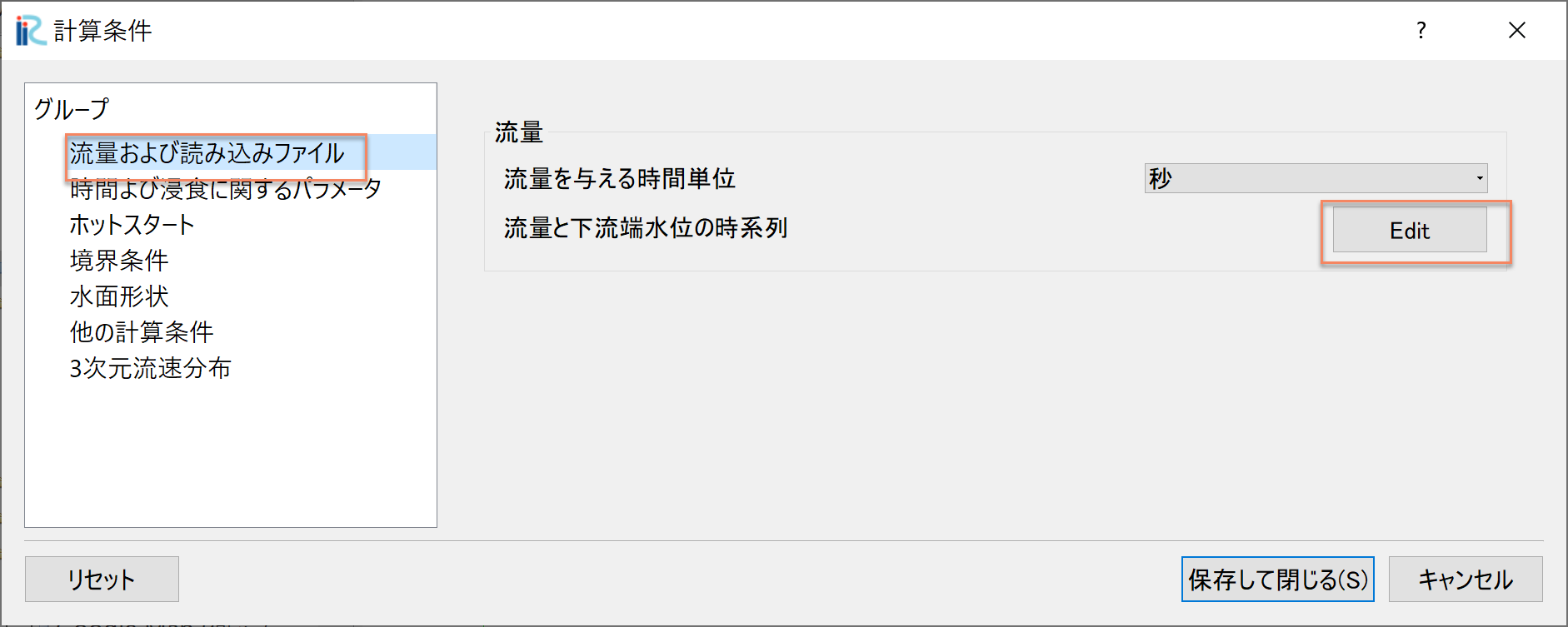
Figure 13 :流量設定
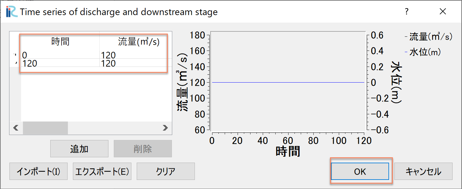
Figure 14 :流量下流端水位設定ウィンドウ
Figure 14 において,「時間」「流量」のハイドログラフを入力する. ここでは,0~120秒まで,120㎥/sの一定流量を与える.設定が終わったら[OK]を押して ウィンドウを閉じる.
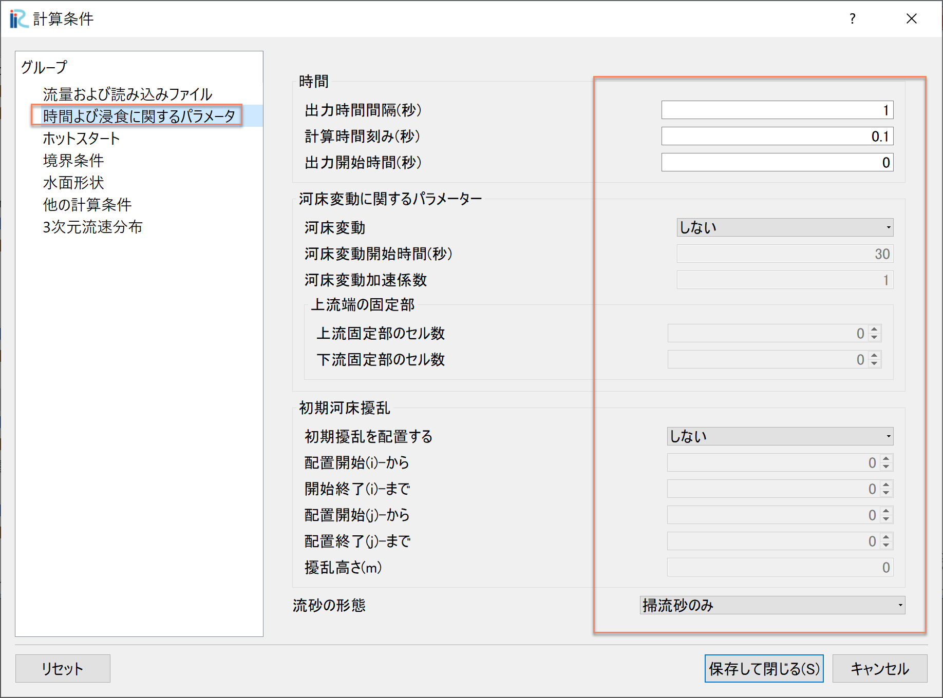
Figure 15 :時間および浸食に関するパラメータ
「時間および浸食に関するパラメーター」は Figure 15 のように設定する.
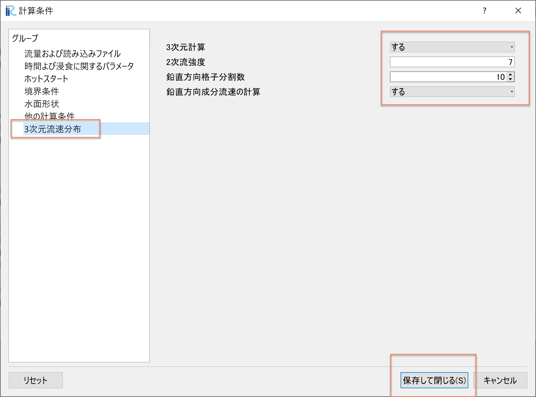
Figure 16 :3次元流速分布
「ホットスタート」「境界条件」「水面形状」「他の計算条件」はデフォルトのままとし, 「3次元流速分布]は, Figure 16 のように設定して 「保存して閉じる」をクリックする.
計算の実行

Figure 17 :計算実行中の画面
[計算]→[実行]を指定すると,「保存しますか?」など聞かれるので, 特別な理由が無い限りは「はい(Y)」を選択すると,計算が実行され, 終了すると,Figure 17 のような画面が現れる. ここで,[OK]を押して,計算は終了となる.
計算結果の表示
計算の終了後,[計算結果]→[新しい可視化ウィンドウ(2D)を開く]を選ぶことによって,可視化ウィンドウが現れる.
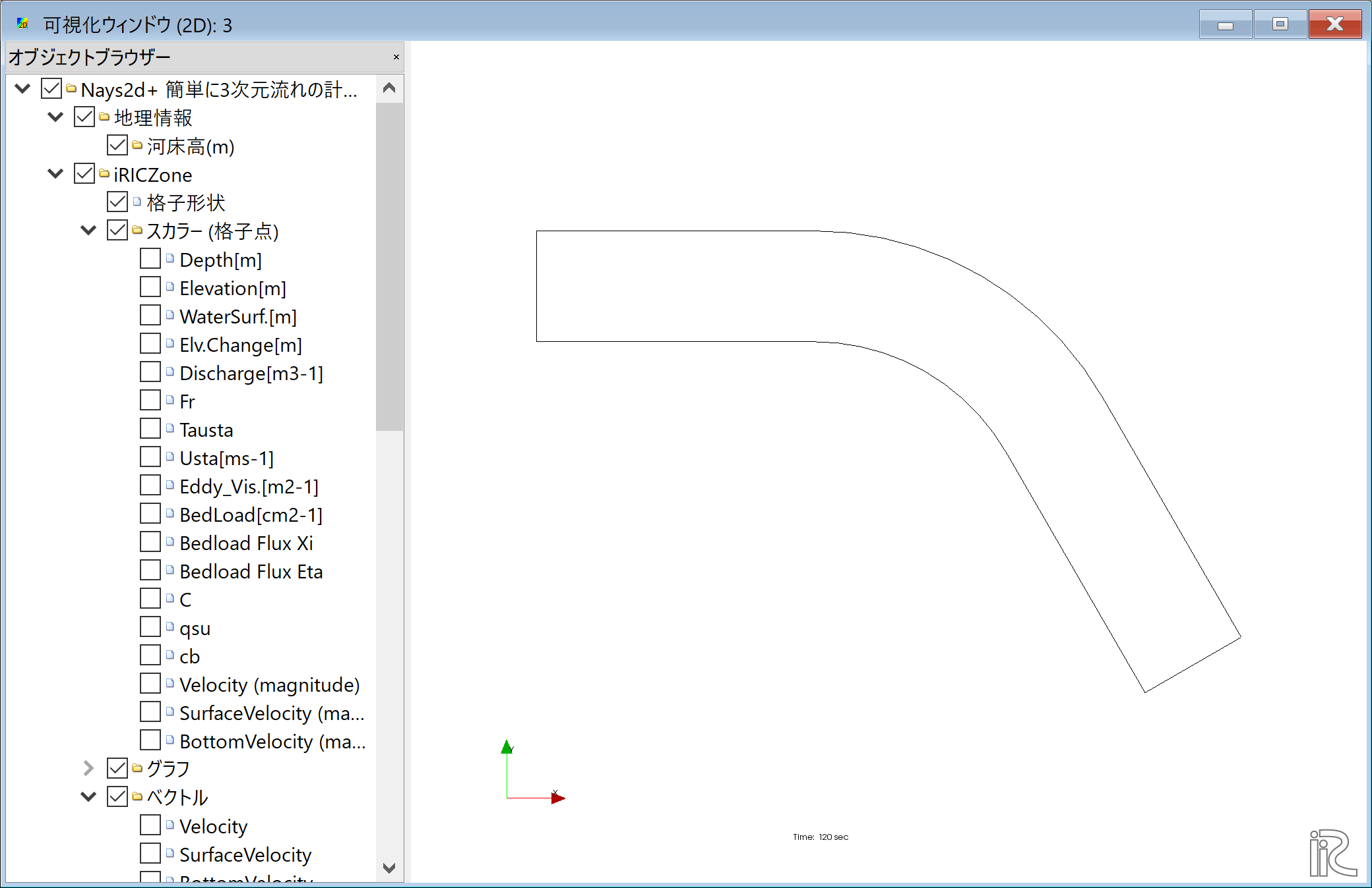
Figure 18 : 計算結果の表示(1)
「Ctrl」ボタンとマウス右ボタンを押しながらマウスを上下左右に動かすことによって, 3次元的な見え方が,また,マウスぼセンターダイヤを回すことにより, Figure 19 のような 拡大・縮小が可能となっている.
Figure 19 : 3D格子の移動・拡大・縮小
水深の表示
オブジェクトブラウザーで,「スカラー(格子点)」の「Depth」に☑マークを入れて, 右クリックして[プロパティ]をクリックすると, 「スカラー設定」ウィンドウ Figure 20 が現れる.
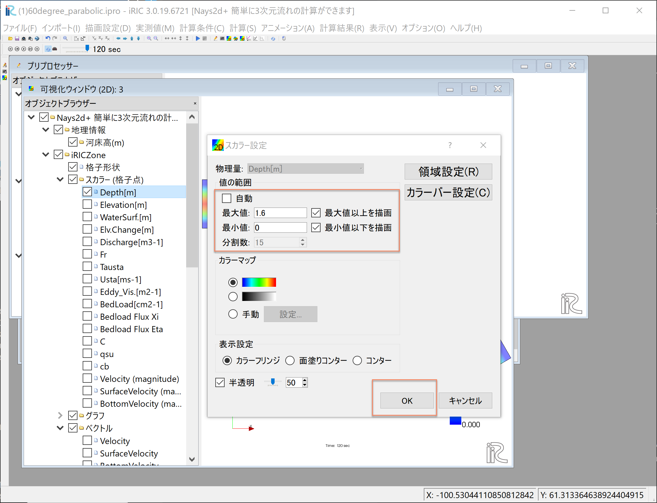
Figure 20 : スカラーの設定
Figure 20 の赤囲いの部分の設定をして,[OK]をクリックすると Figure 21 が表示される.ここでカラーバーはオブジェクトブラウザーで「Depth」を押した状態で, 左マウスで移動出来る.縦横の変更も可能である.また,時刻表示のフォントの変更も オブジェクトブラウザーの「時刻」「プロパティ」で可能である.( Figure 22 参照.) .
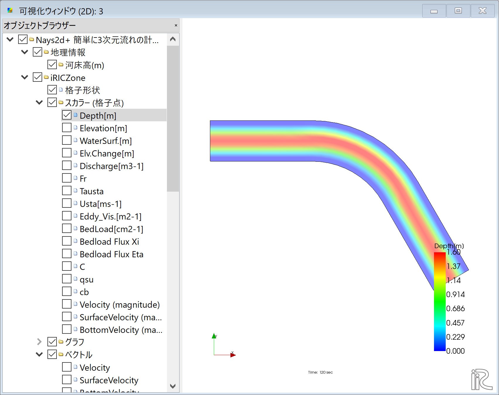
Figure 21 : 水深の表示
Figure 22 : カラバーの移動と時刻表示のサイズ変更
流速ベクトルの表示
オブジェクトブラウザーで,[ベクトル][Velocity]に☑マーク入れて, [ベクトル]をフォーカスさせてマウス右ボタン[プロパティ]をクリックすると, 「ベクトル設定」ウィンドウ Figure 23 が現れる.ここで,赤丸の設定をして[OK]を 押すと Figure 24 が表示される. Figure 24 は水深平均流速ベクトルである.
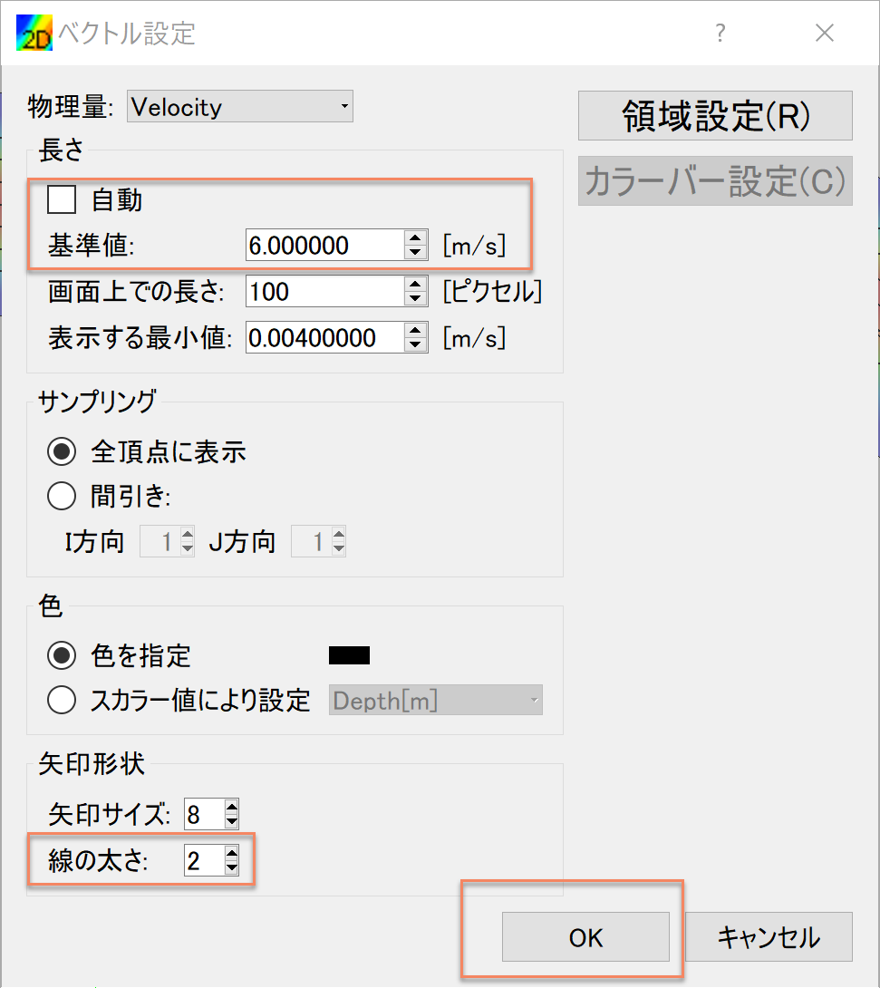
Figure 23 : ベクトル設定
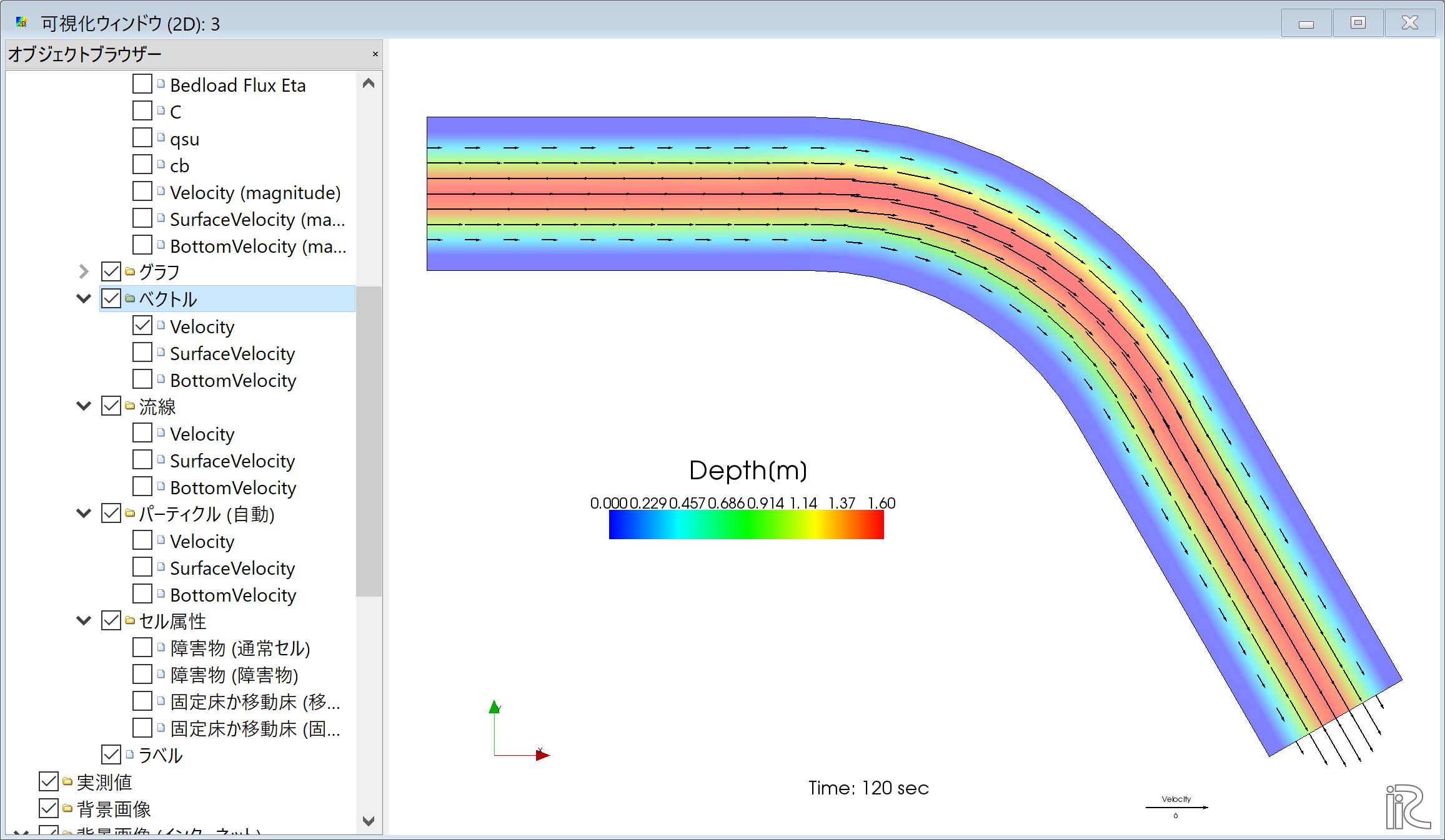
Figure 24 : 水深平均流速ベクトル表示
Figure 24 の状態で,オブジェクトブラウザーの「ベクトル」の「SurfaceVelocity」に ☑マークを入れると「表面流速ベクトル」 Figure 25 が,また, 「BottomVelocity」に☑マークを入れると 「底面近傍流速」 Figure 26 が表示される.
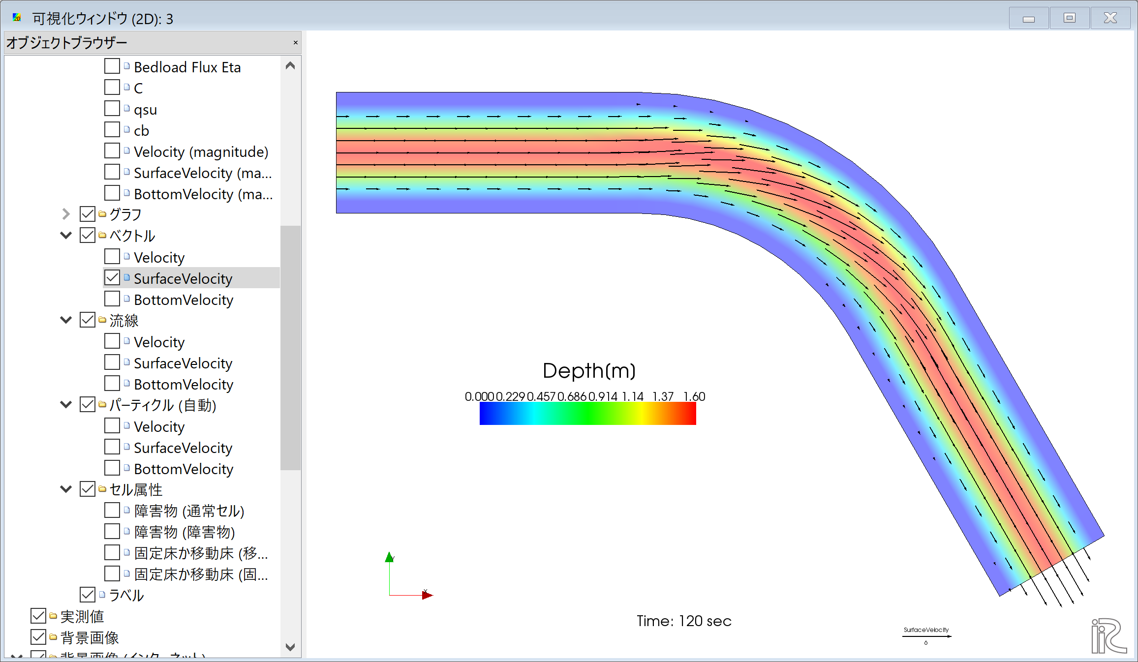
Figure 25 : 表面流速ベクトル表示
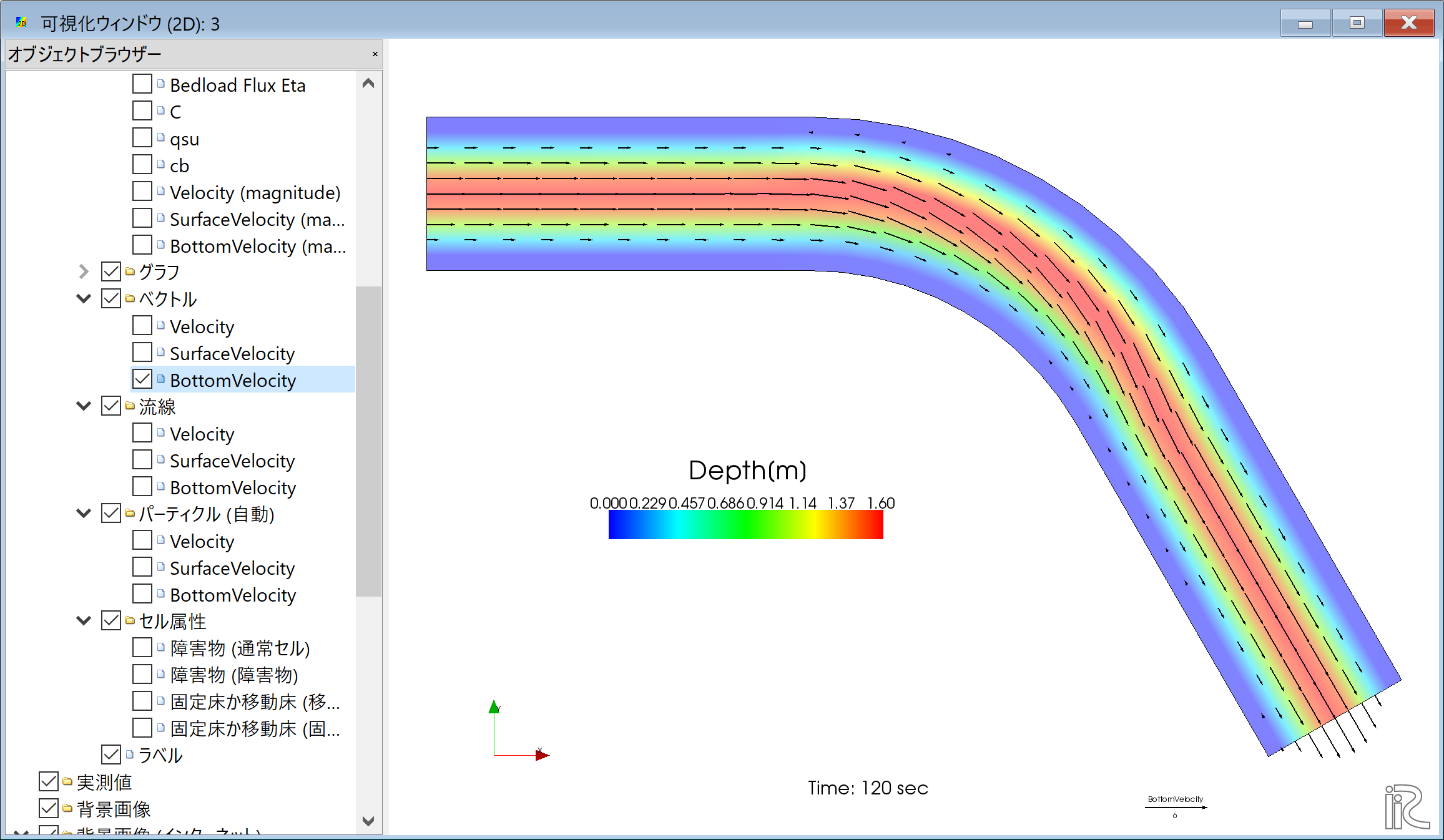
Figure 26 : 河床近傍流速ベクトル表示
Figure 24 ,Figure 25 , Figure 26 を比較すると, 明らかに水深平均流速は流路に平行,表面流速は外岸向き,底面流速は内岸向きになっており, 湾曲部の2次流が計算されていることが分かる.
流線の表示
オブジェクトブラウザーの「ベクトル」を一旦アンチェックし,「流線」に☑マークを入れる. 「Velocity」に☑マークを入れると「水深平均流速」による流線 Figure 27 が, 「SurfaceVelocity」に☑マークを入れると「表面流速」による流線 Figure 28 が, 「BottomVelocity」に☑マークを入れると「底面近傍流速」による流線 Figure 29 が 表示される.
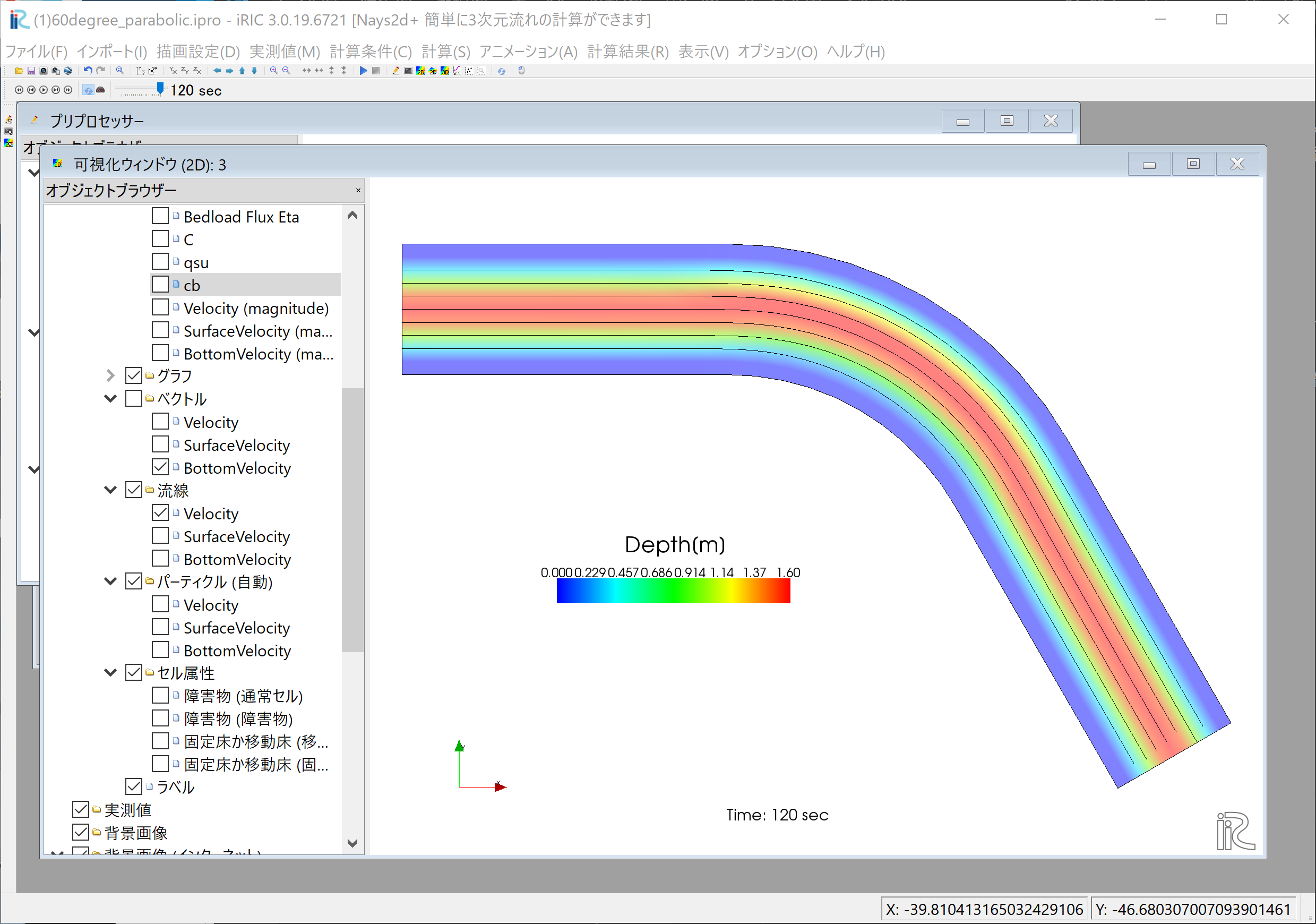
Figure 27 : 水深平均流速による流線
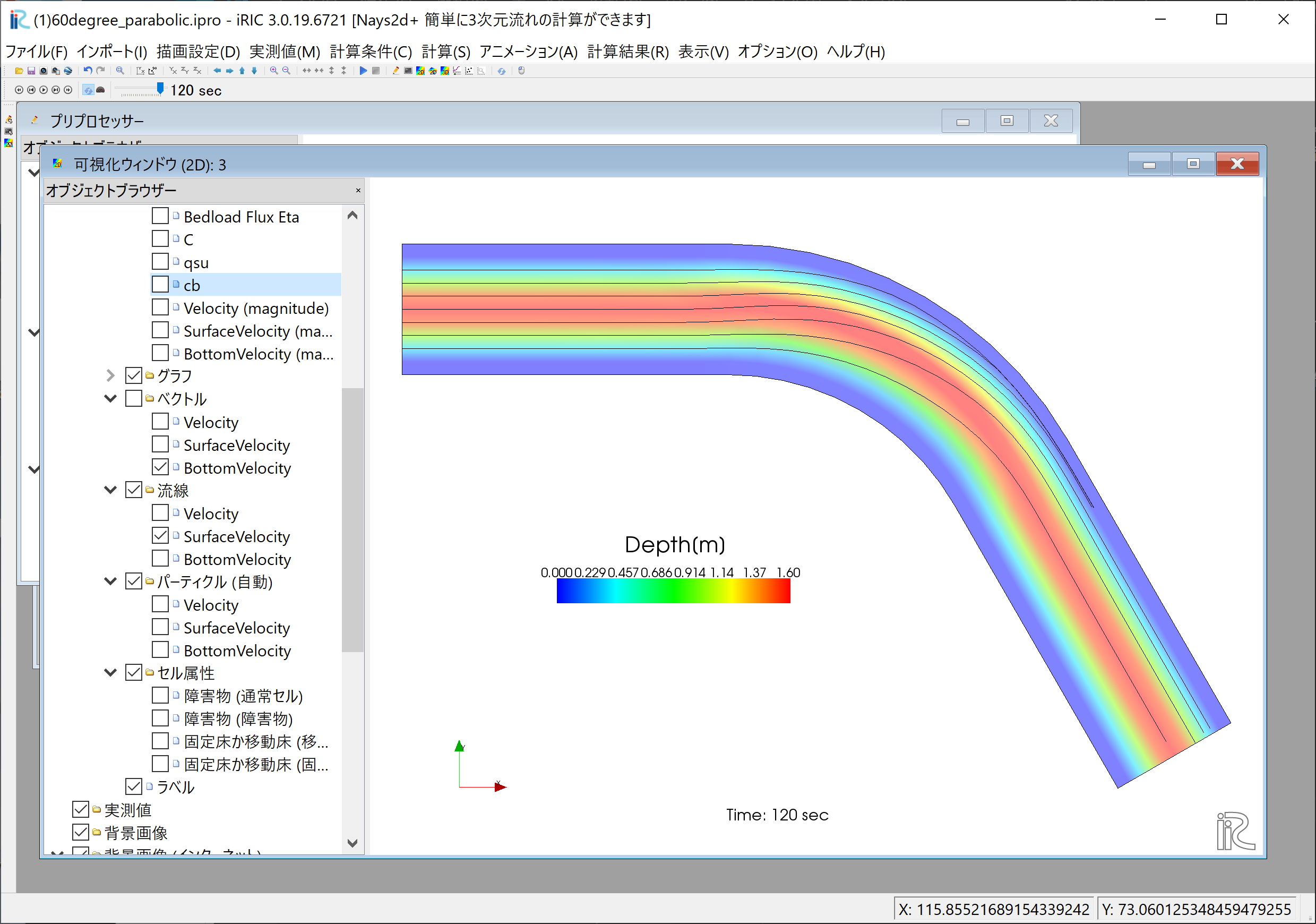
Figure 28 : 表面流速による流線
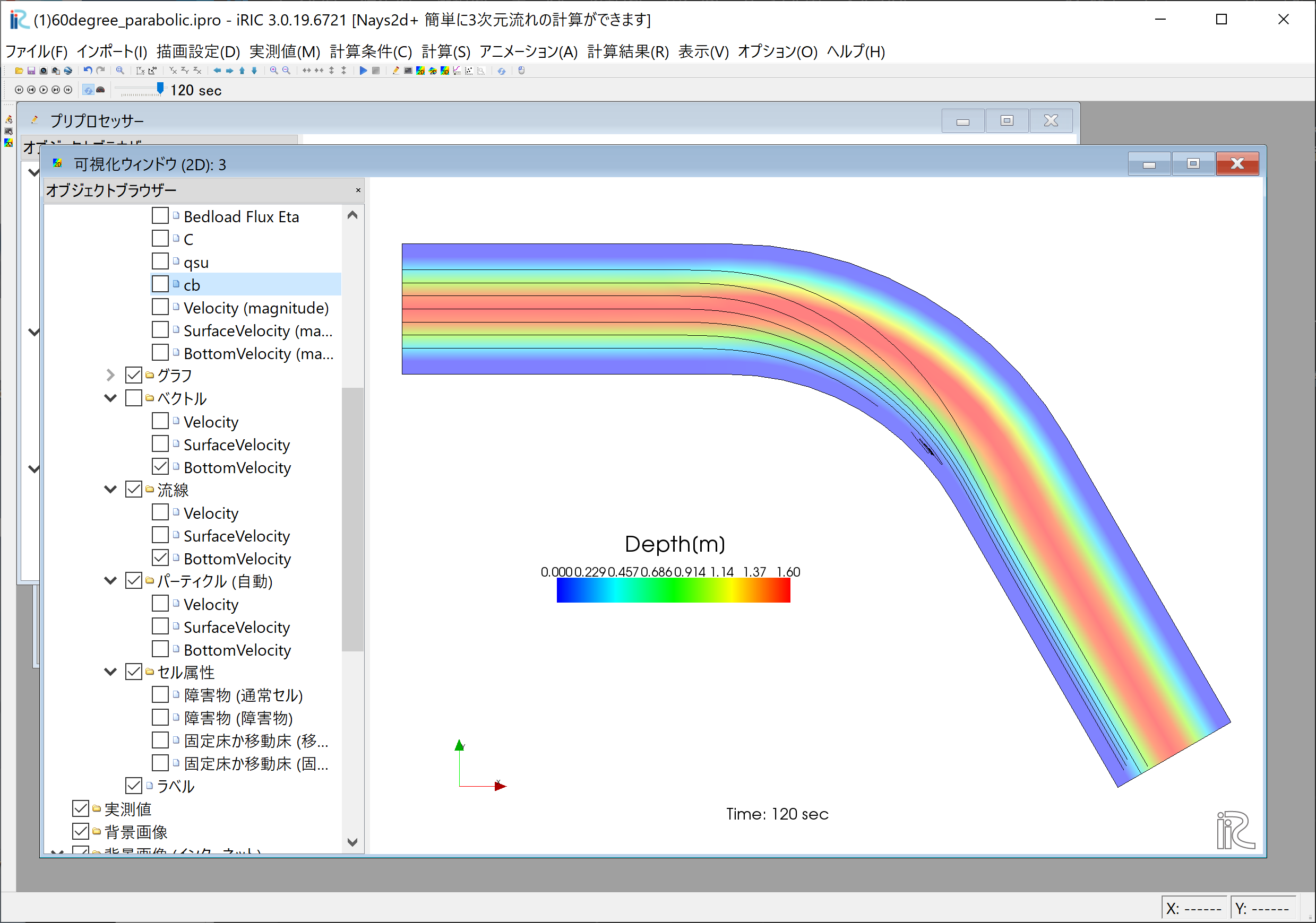
Figure 29 : 河床近傍流速による流線
ベクトルと同様に,湾曲部の2次流の影響が計算されている.