[計算例 2] 360°円形水路における流れ
Nays2d+を用いて,360°円形水路の流れの計算を行う.
計算格子の作成
計算格子の作成は[2次元円弧形水路格子生成ツール]を用いる. Figure 30 で[Nays3dv用格子生成ツール]を選択し.[OK]をクリックする.
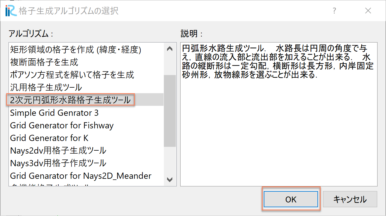
Figure 30 : 格子生成アルゴリズムの選択
下図の Figure 31 で赤囲いの部分を設定し,格子生成をクリックすると. Figure 32 が表示され「マッピングを実行しますか?」と聞かれるので, [はい(Y)]をクリックすると,格子が表示される.
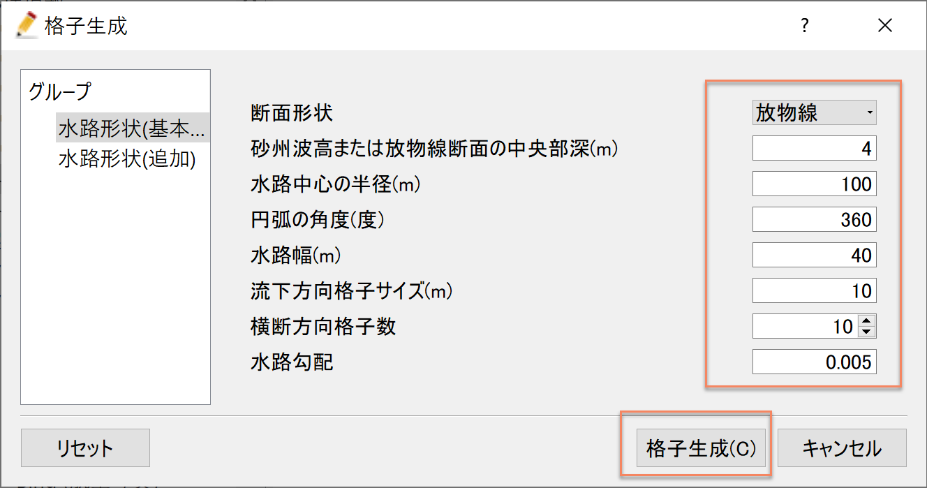
Figure 31 : 格子生成: 水路形状(基本)
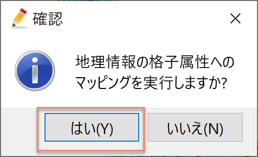
Figure 32 : マッピングの実行
格子が表示されたら,「格子」「格子点の属性」「河床高」に☑マークを入れると 放物線断面で一定勾配の360°円形水路の格子が生成されたことが確かめられる. ( Figure 33 )
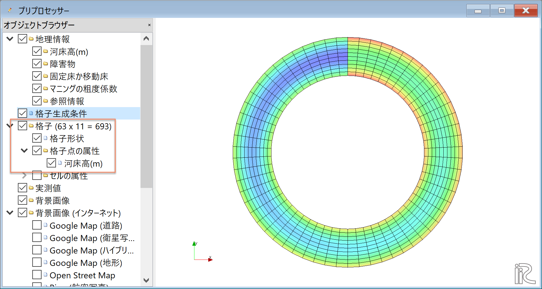
Figure 33 : 格子生成の完了
計算条件の設定
メニューバーから[計算条件]→[設定]を選ぶと「計算条件」入力用のウィンドウが表示される ( Figure 34 )
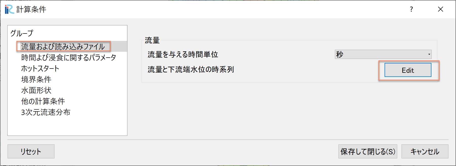
Figure 34 : 計算条件:モデルパラメータ
「計算条件」ウィンドウ Figure 34 の「流量および読み込みファイル」で [Edit]をクリックし,
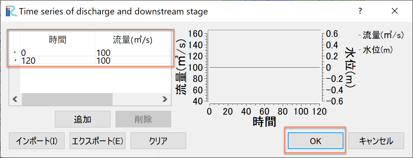
Figure 35 : 計算条件:流量ハイドログラフ設定
「流量ハイドログラフ設定」ウィンドウで Figure 35 のように設定するし, [OK]をクリックする.
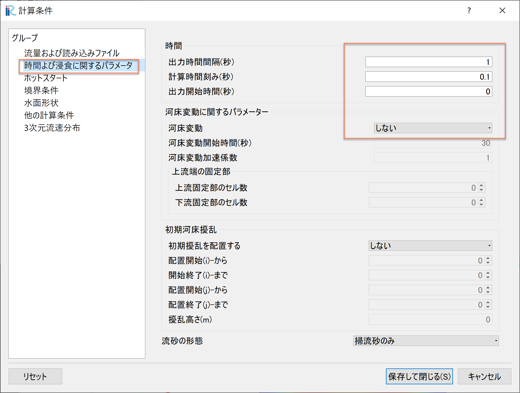
Figure 36 : 計算条件:時間および繰り返し計算パラメーター
「グループ」の「時間および浸食に関するパラメーター」は Figure 36 のように設定する.
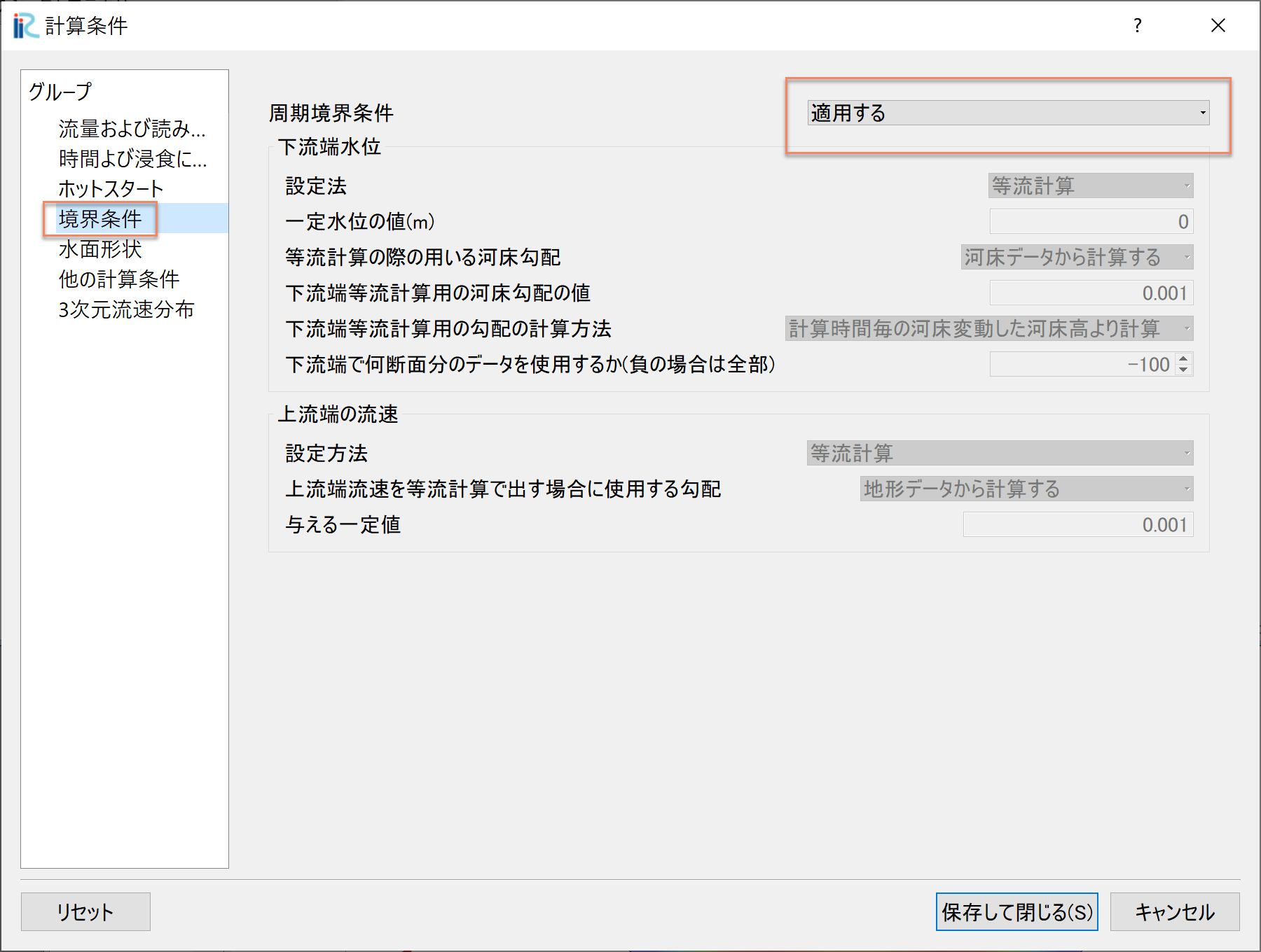
Figure 37 : 計算条件:境界条件
「グループ」「境界条件」の「周期境界条件」は,無限に続く円形水路の計算なので, 「適用する」に設定する.
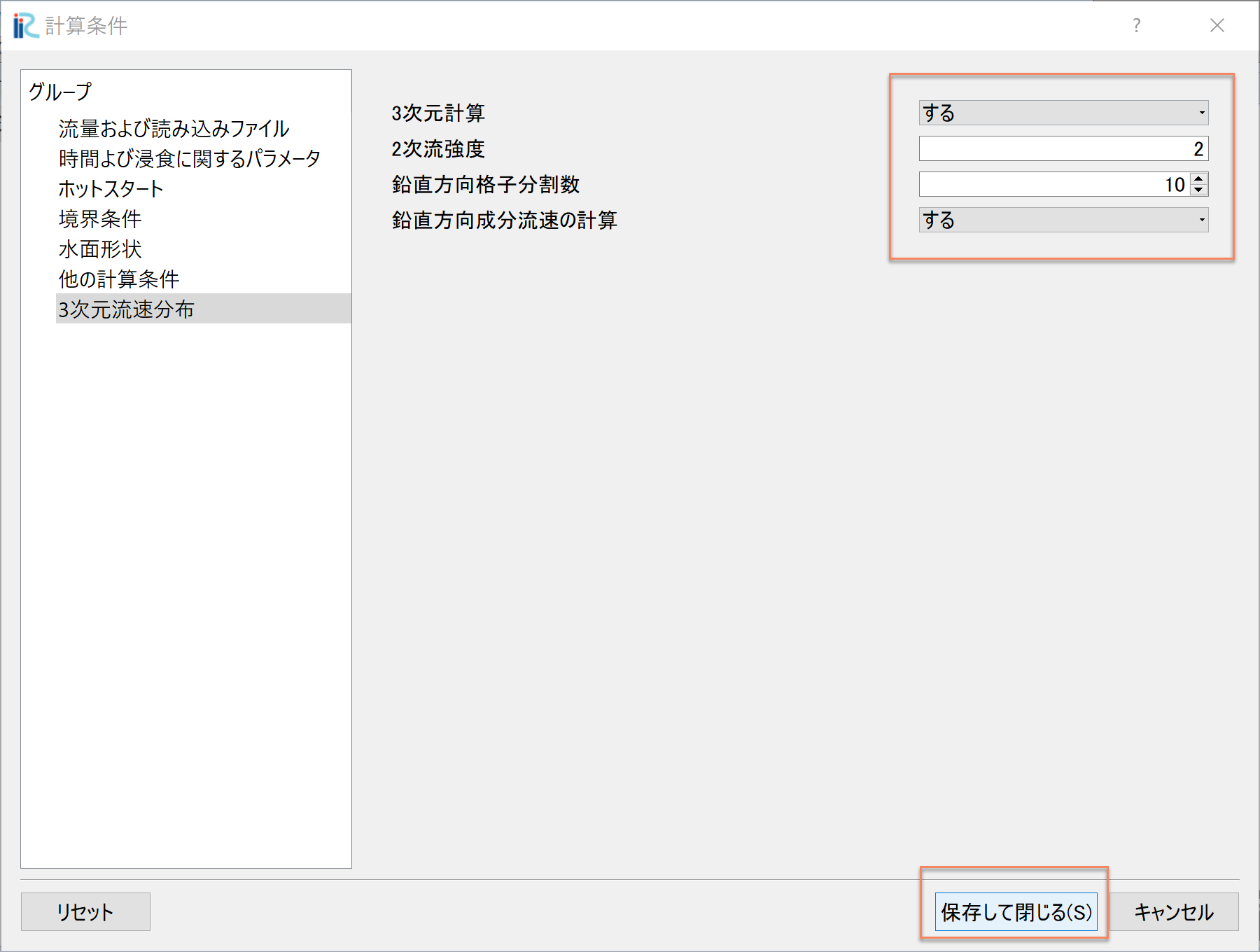
Figure 38 : 計算条件:3次元流速分布
「グループ」「3次元流速分布」の設定は Figure 38 のように設定して 「保存して閉じる」をクリックする.
計算の実行
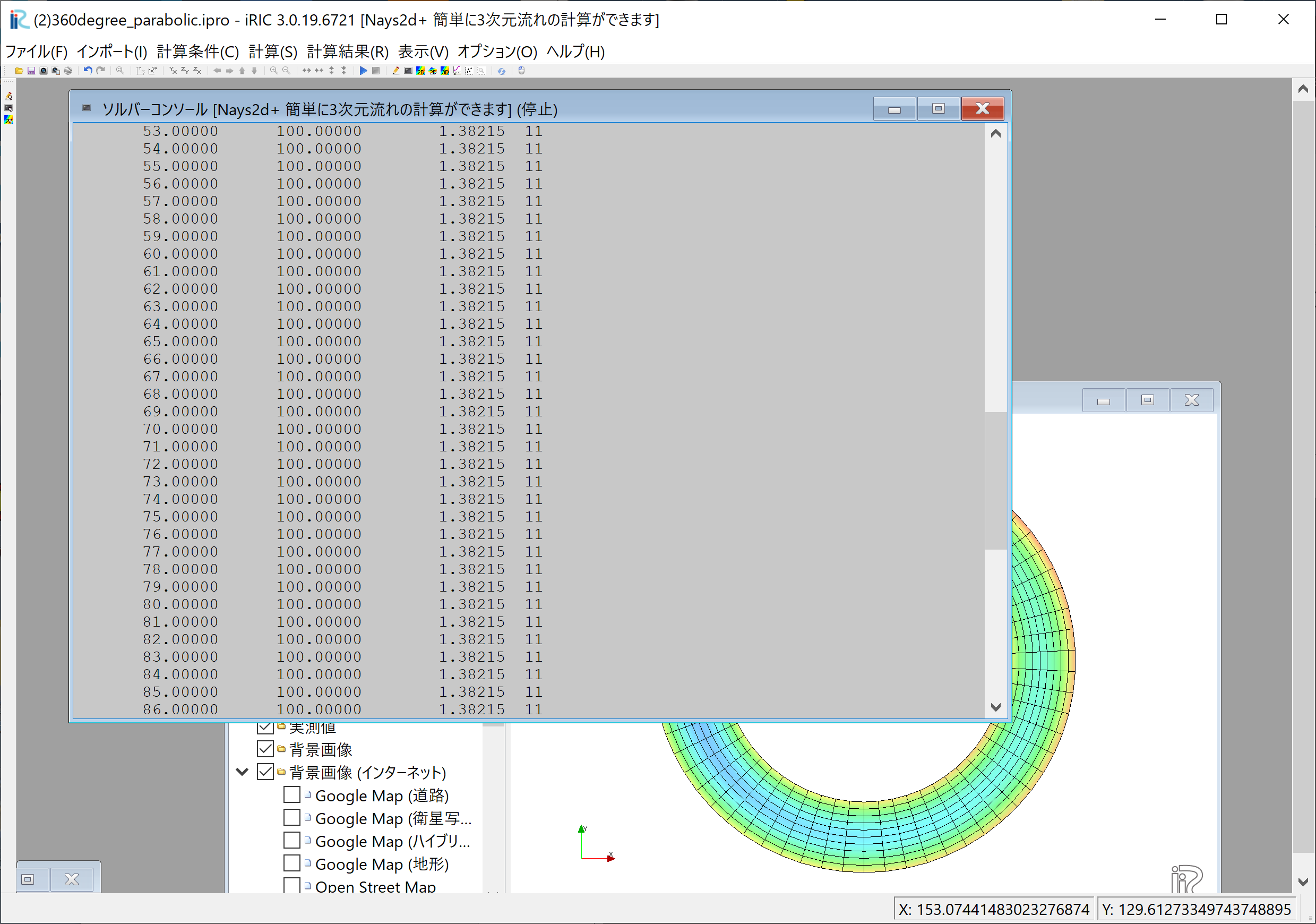
Figure 39 :計算実行中の画面
[計算]→[実行]を指定すると,Figure 39 のような画面が現れ計算が始まる.
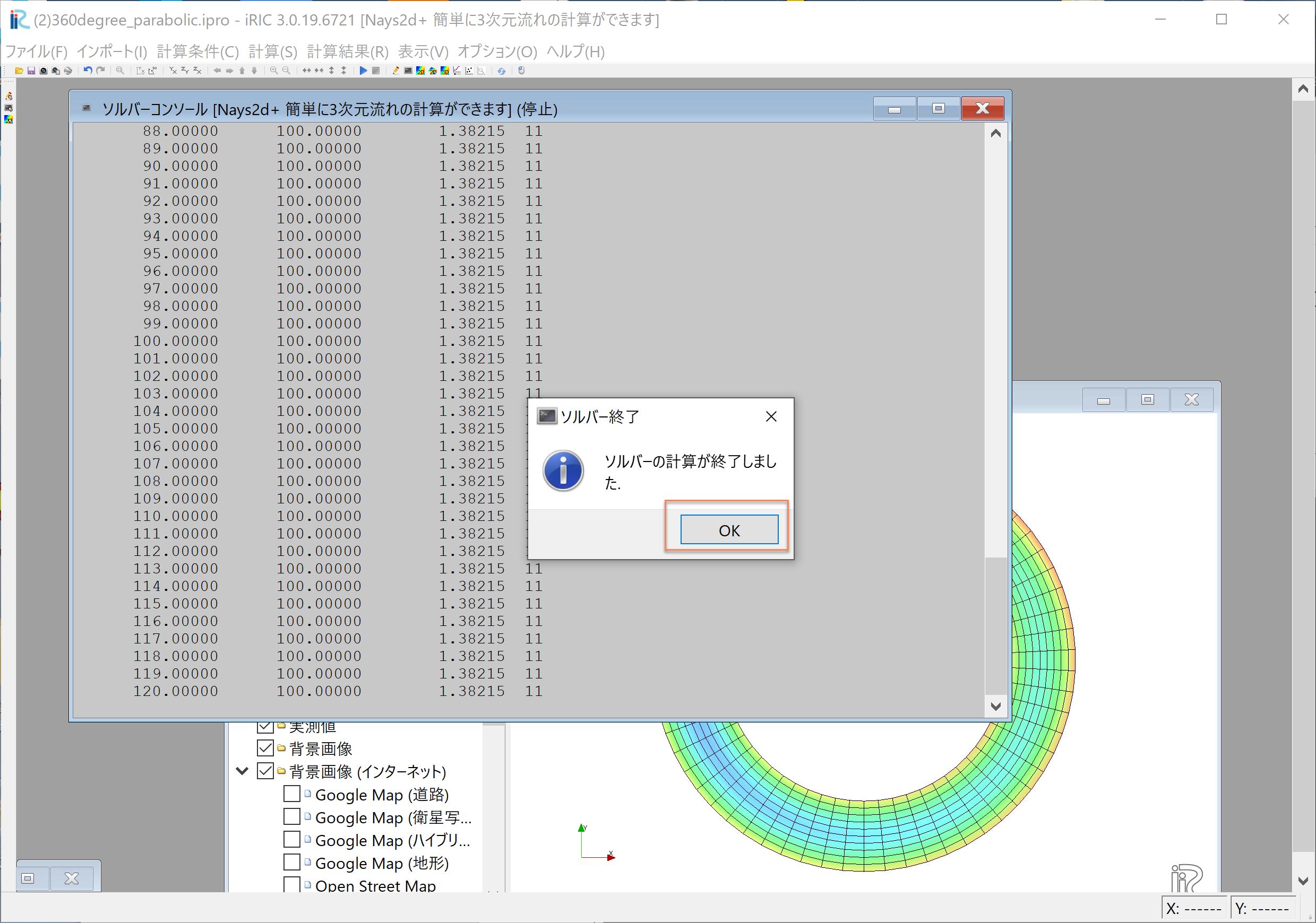
Figure 40 :計算の終了
計算が終了すると, Figure 40 のような表示がされる.
計算結果の表示
計算の終了後,[計算結果]→[新しい可視化ウィンドウ(2D)を開く]を選ぶことによって,可視化ウィンドウが現れる.
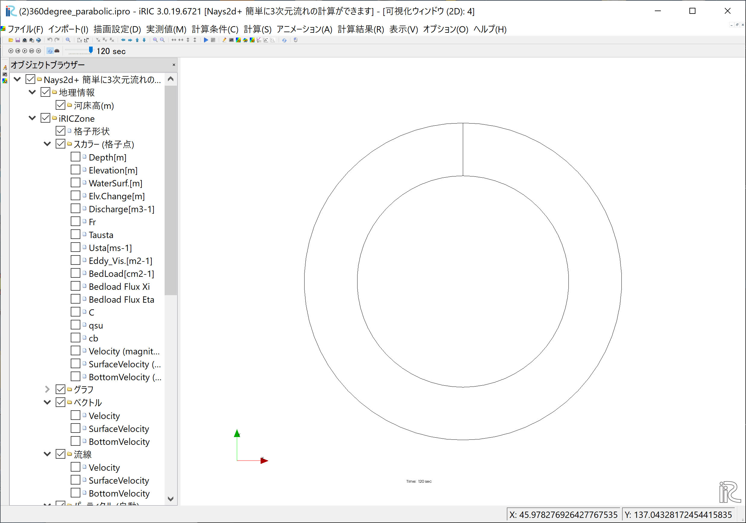
Figure 41 : 計算結果の表示(1)
水深の表示
オブジェクトブラウザーで,「スカラー(格子点)」の「Depth」に☑マークを入れて, 右クリックして[プロパティ]をクリックすると, 「スカラー設定」ウィンドウ Figure 42 が現れる.
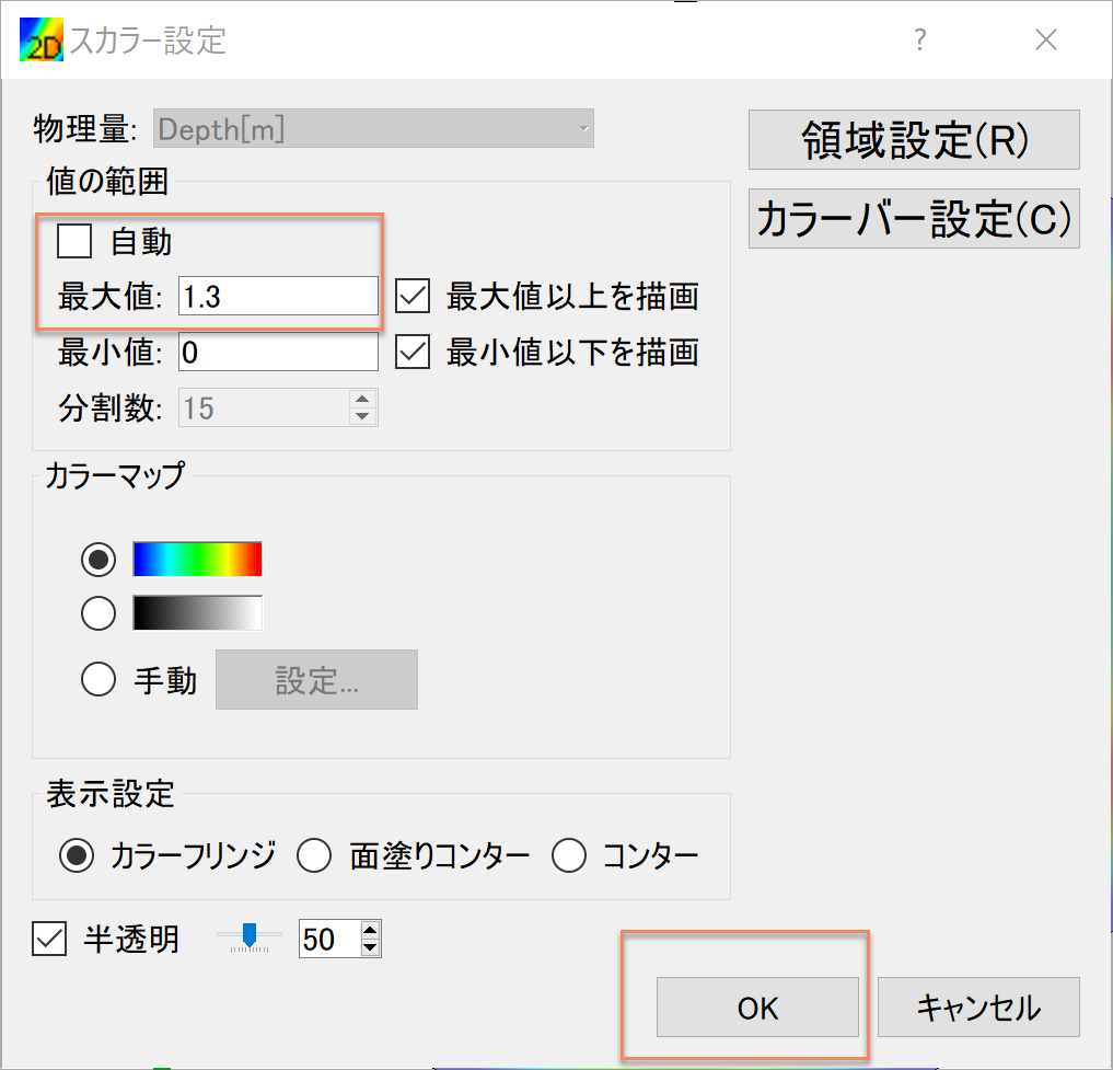
Figure 42 : スカラーの設定
Figure 42 の赤囲いの部分の設定をして,[OK]をクリックすると Figure 43
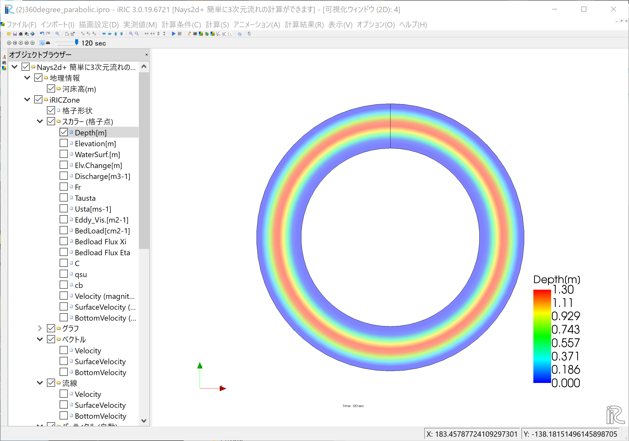
Figure 43 : 水深の表示
流速ベクトルの表示
オブジェクトブラウザーで,[ベクトル][Velocity]に☑マーク入れて, [ベクトル]をフォーカスさせてマウス右ボタン[プロパティ]をクリックすると, 「ベクトル設定」ウィンドウ Figure 44 が現れる.ここで,赤丸の設定をして[OK]を 押すと Figure 45 が表示される. Figure 45 は水深平均流速ベクトルである.
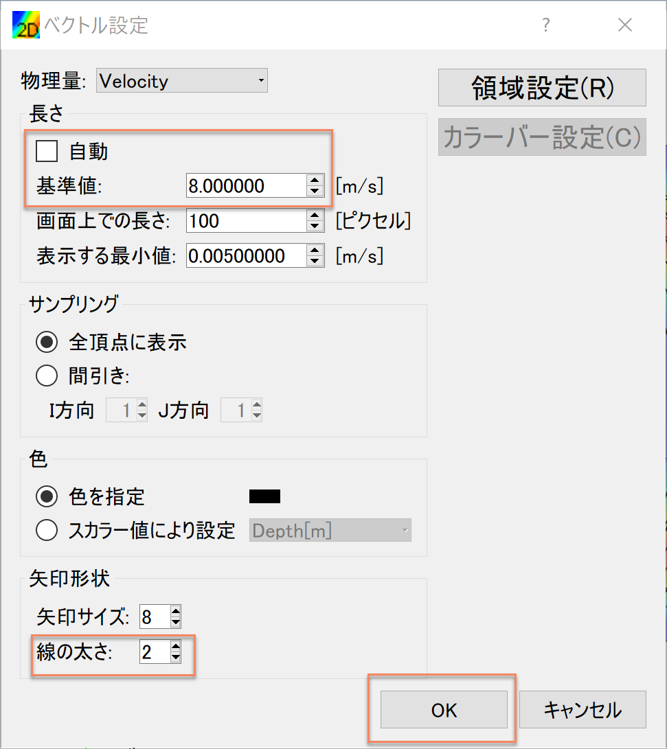
Figure 44 : ベクトル設定
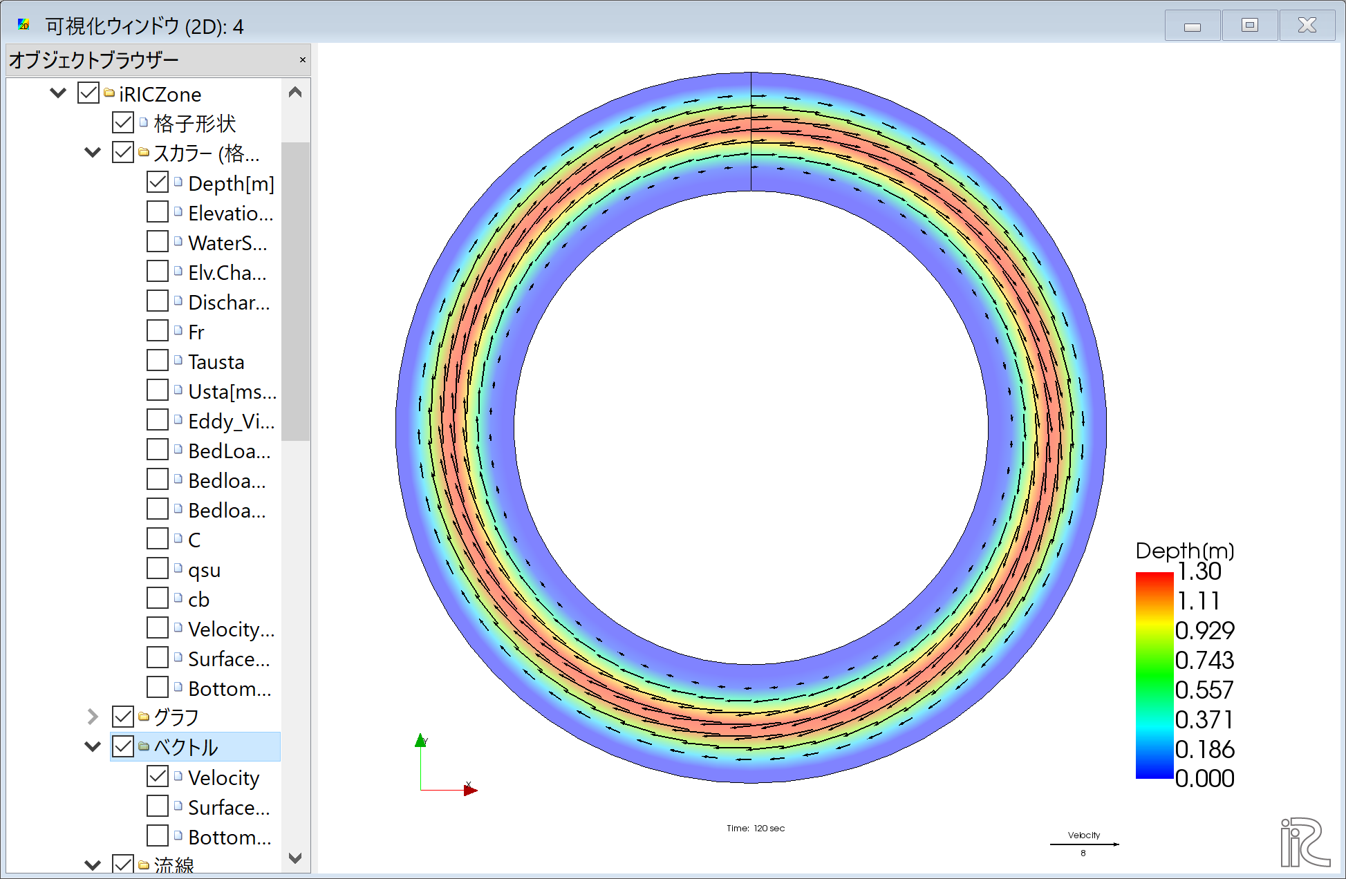
Figure 45 : 水深平均流速ベクトル表示
Figure 45 の状態で,オブジェクトブラウザーの「ベクトル」の「SurfaceVelocity」に ☑マークを入れると「表面流速ベクトル」 Figure 46 が,また, 「BottomVelocity」に☑マークを入れると 「底面近傍流速」 Figure 47 が表示される.
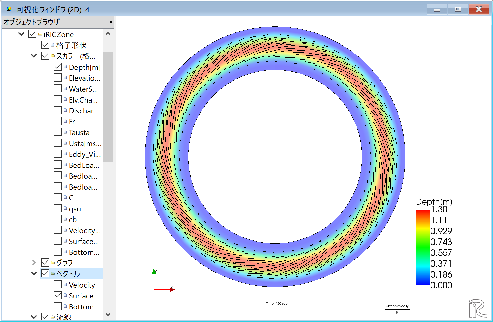
Figure 46 : 表面流速ベクトル表示
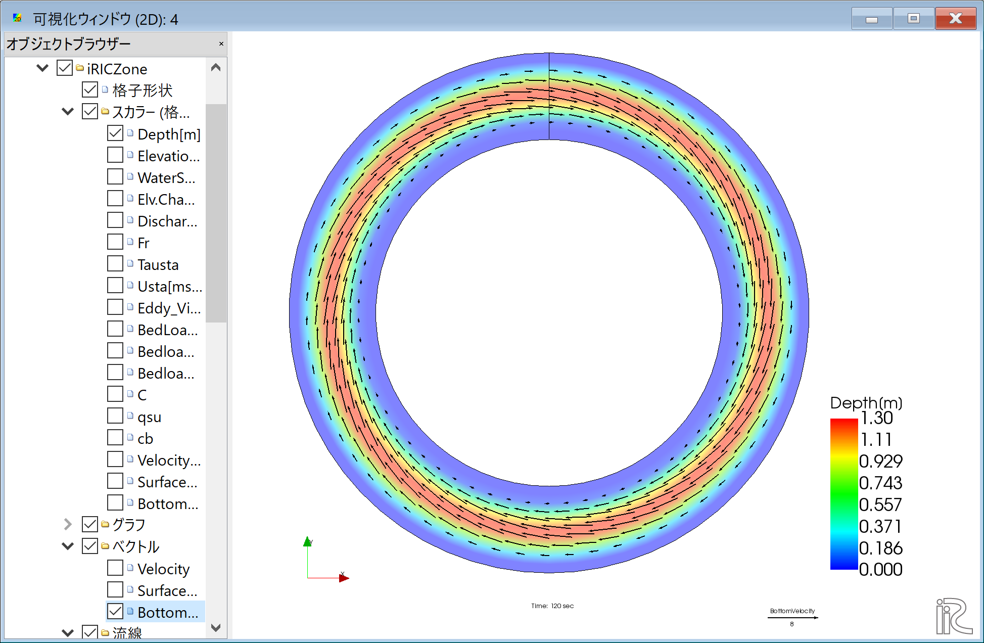
Figure 47 : 河床近傍流速ベクトル表示
Figure 45 ,Figure 46 , Figure 47 を比較すると, 明らかに水深平均流速は流路に平行,表面流速は外岸向き,底面流速は内岸向きになっており, 湾曲部の2次流が計算されていることが分かる.
流線の表示
オブジェクトブラウザーの「ベクトル」を一旦アンチェックし,「流線」に☑マークを入れる. 「Velocity」に☑マークを入れると「水深平均流速」による流線 Figure 48 が, 「SurfaceVelocity」に☑マークを入れると「表面流速」による流線 Figure 49 が, 「BottomVelocity」に☑マークを入れると「底面近傍流速」による流線 Figure 50 が 表示される.
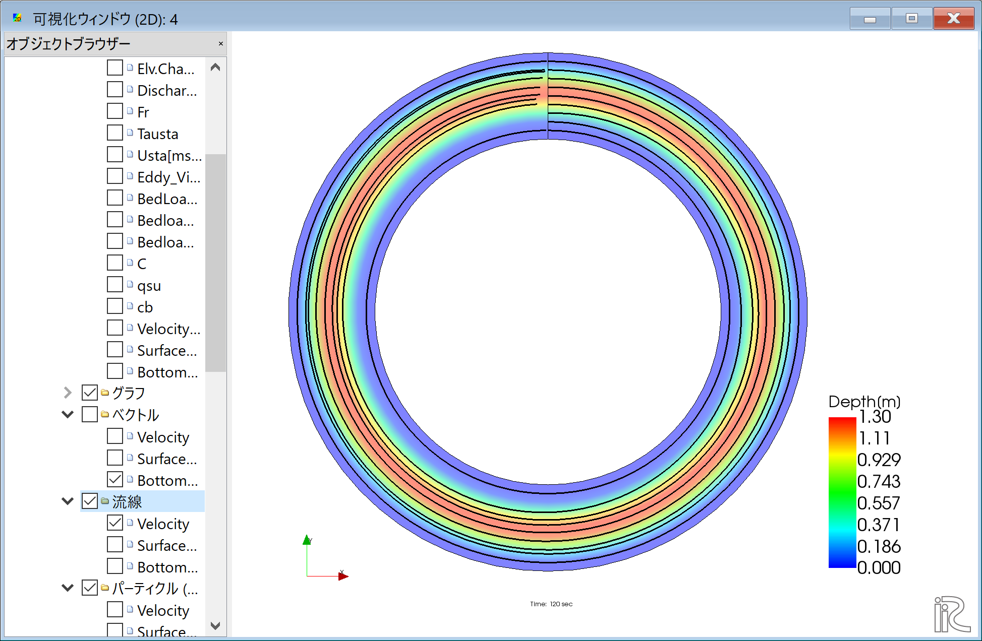
Figure 48 : 水深平均流速による流線
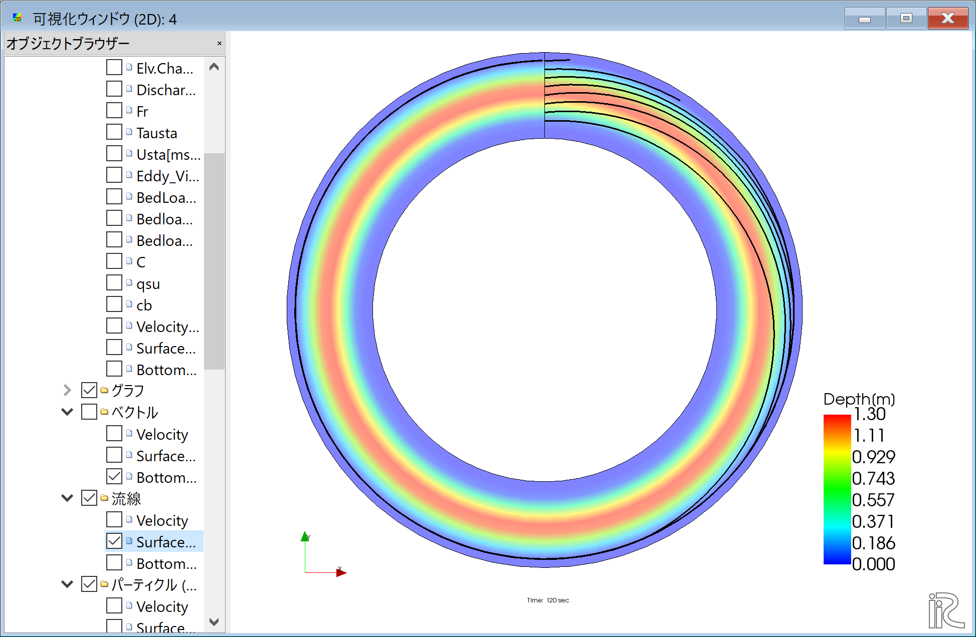
Figure 49 : 表面流速による流線
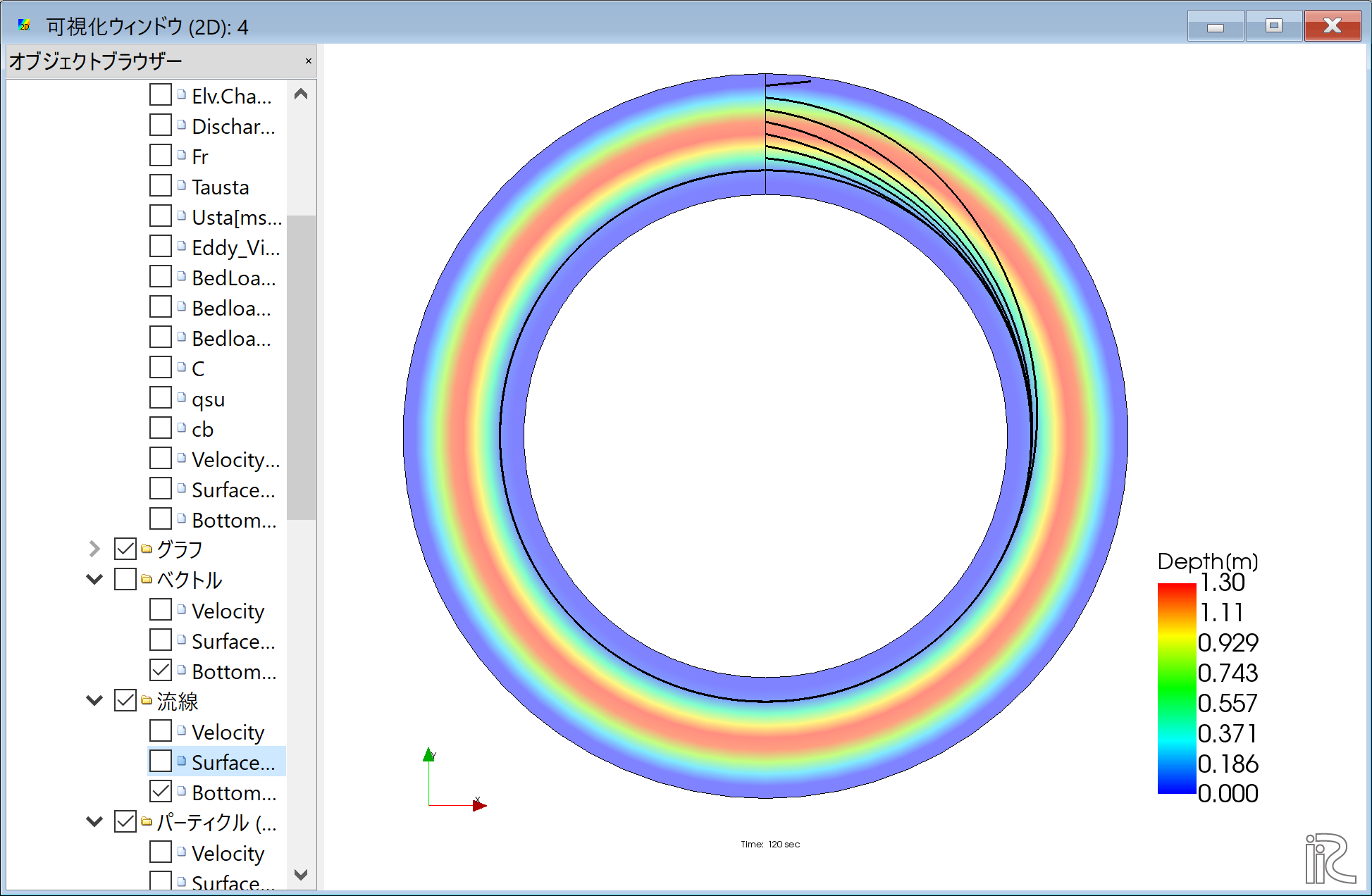
Figure 50 : 河床近傍流速による流線
ベクトルと同様に,湾曲部の2次流の影響が計算されている.