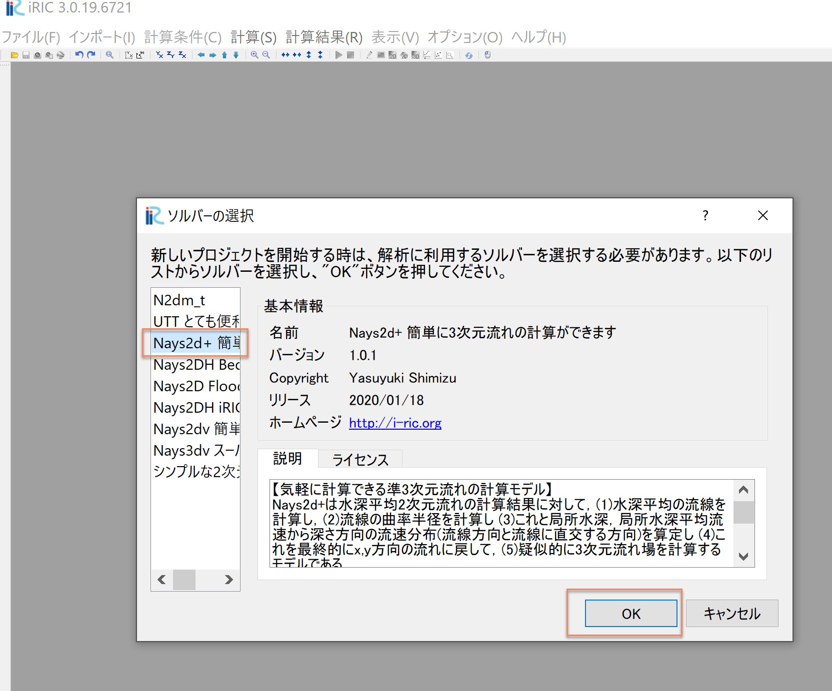
[計算例 5] 実河川における準3次元流れの計算(複断面)
河床高標高データ(横断データ)の読み込み
Figure 123 で「インポート」「河床高」を選択する.
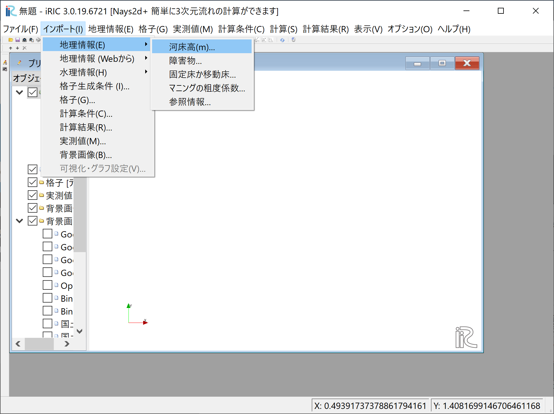
Figure 123 : 河床高ファイル(rivファイル)のインポート
Figure 124 で,「compound.riv」を選択して[開く].(compound.rivは, https://i-ric.org/yasu/fw/rivfiles/compound.riv からダウンロードして ローカルに保存しておくこと).
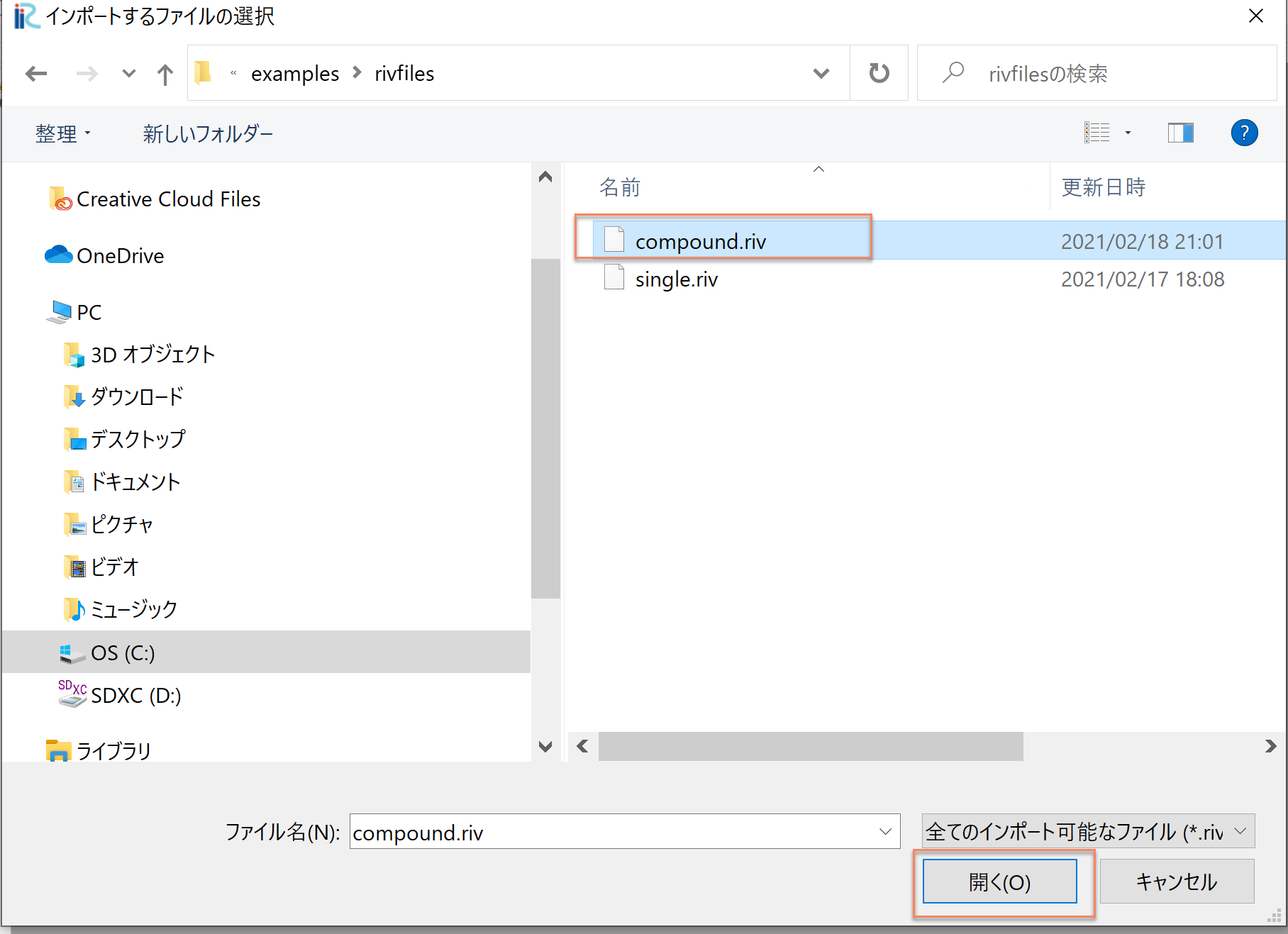
Figure 124 : ファイルの選択
Figure 125 のように「問題が見つかりました」と出るが,構わず[OK]をクリックして 続ける.
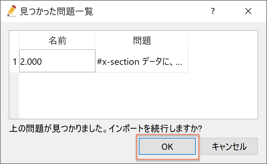
Figure 125 : 見つかった問題
Figure 126 「河川測量データインポート設定」 のウィンドウで, 「左岸と右岸の中点」を選択して[OK]をクリック
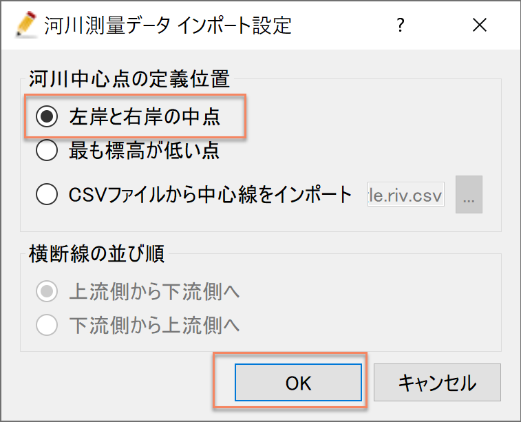
Figure 126 : 河川測量データインポート設定
Figure 127 rivファイルのインポートが完了する. なお,実際の河川のrivfileは横断測量断面そのままの場合,断面どうしの交差の回避や不要部分の 無効化など様々な編集が必要となるが,ここでは編集済みのもの用意してある.実際はそれぞれの 状況に応じた対応が必要となる.
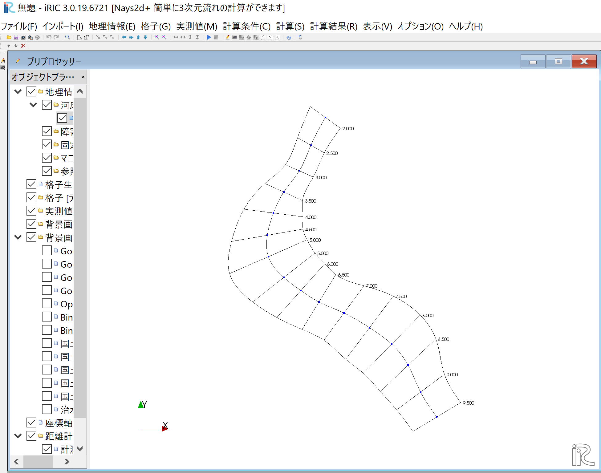
Figure 127 : インポート完了
格子の生成条件の設定
Figure 129 のメニュー画面で,「格子」「格子生成アルゴリズムの選択」を選ぶ
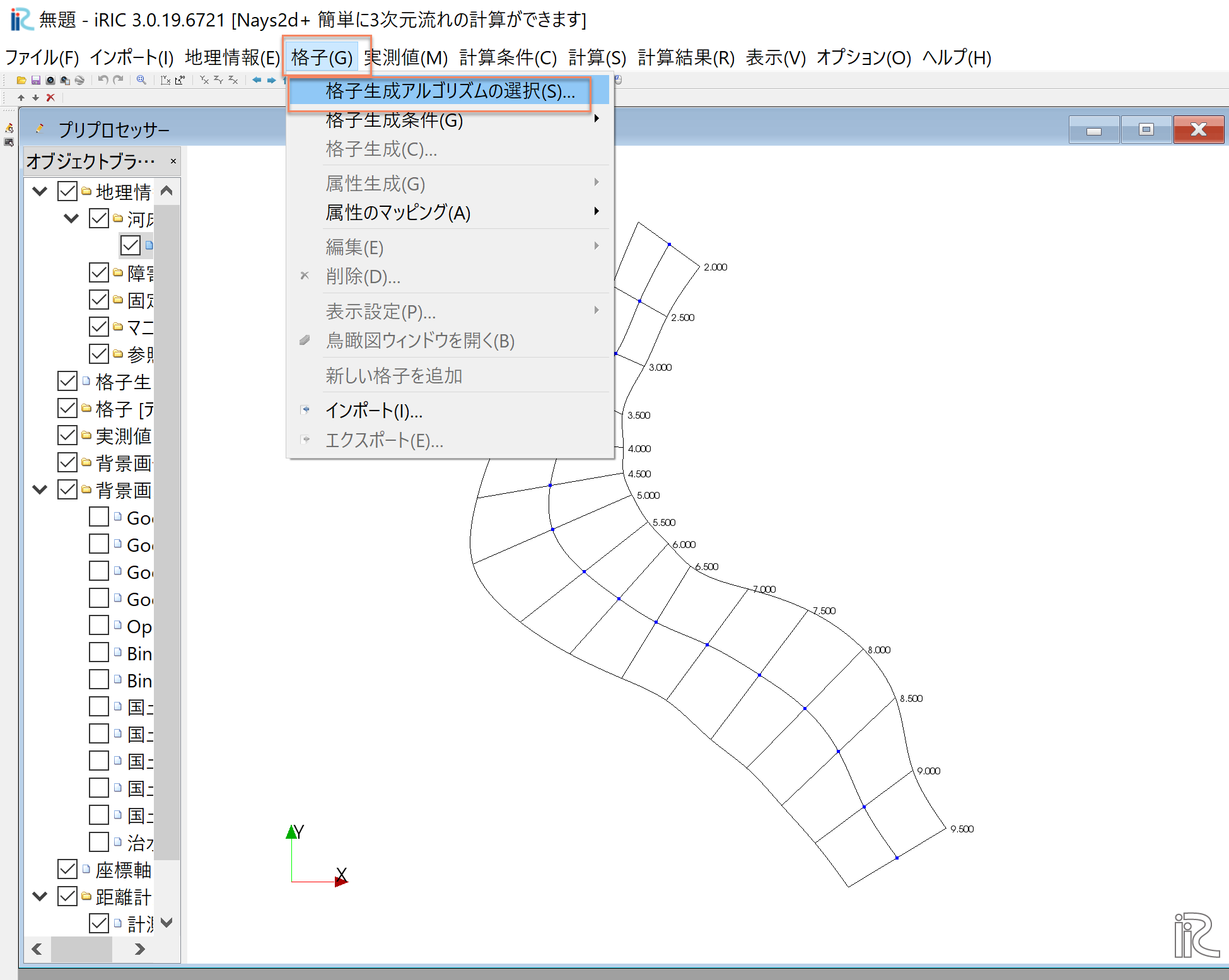
Figure 129 : 格子生成アルゴリズムの選択
Figure 130 「格子アルゴリズムの選択」画面で,「河川測量データから生成」を選んで[OK]をクリック
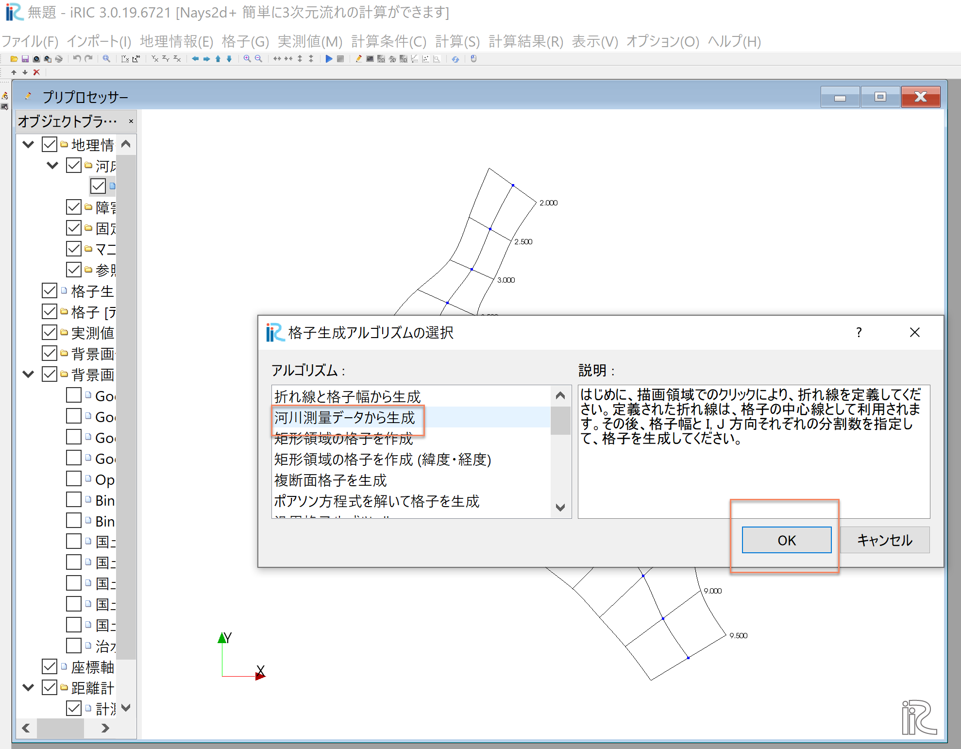
Figure 130 : 河川測量データから生成
Figure 131 格子生成条件設定完了.各横断線の両端とセンターに青丸が表示された画面となる.
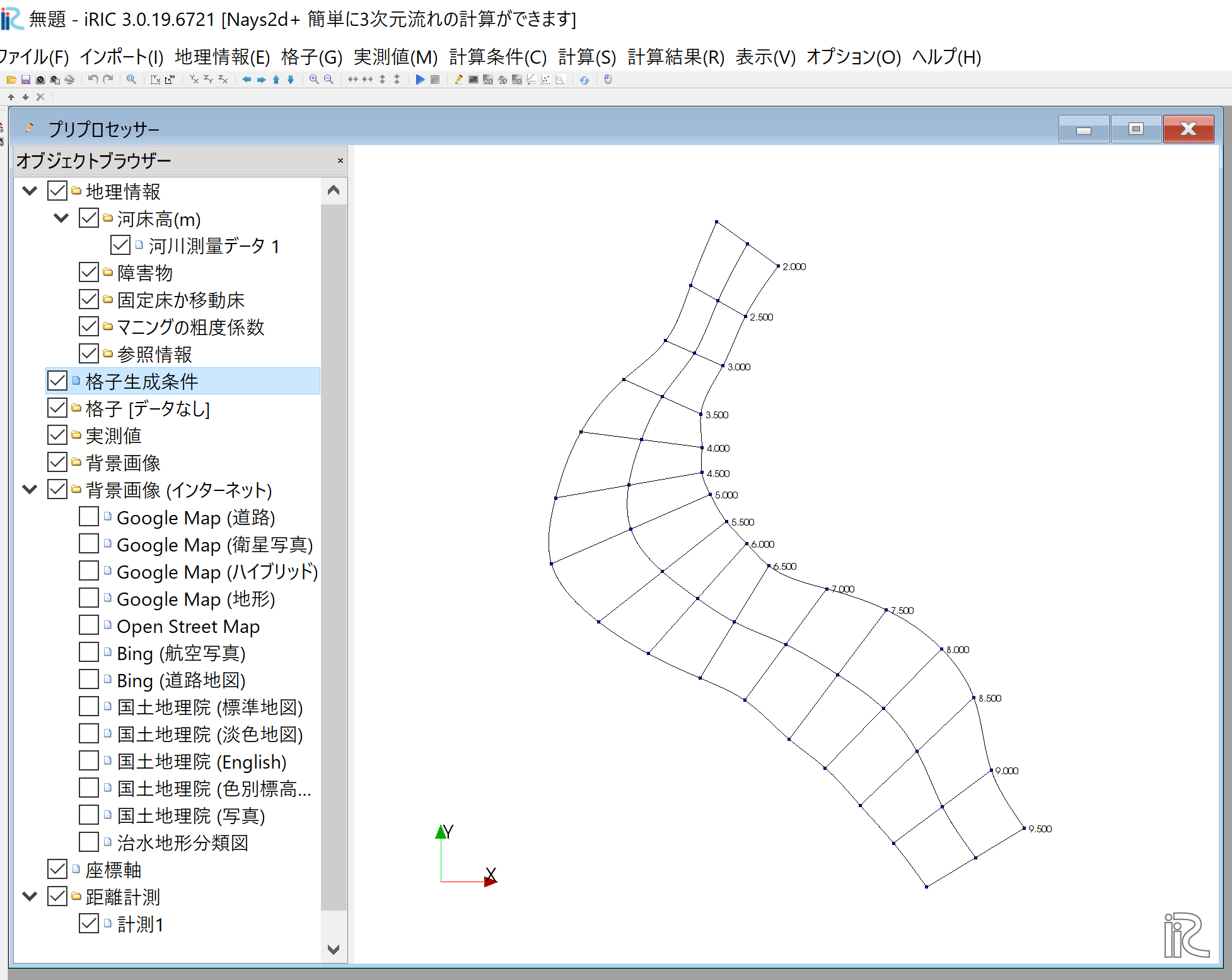
Figure 131 : 格子生成条件設定終了
格子の生成
横断線のうちの一つ(どれでも良い)を選択し,左右岸どちらでも良いので右クリックして, 「分割点の追加(A)」を選択する.
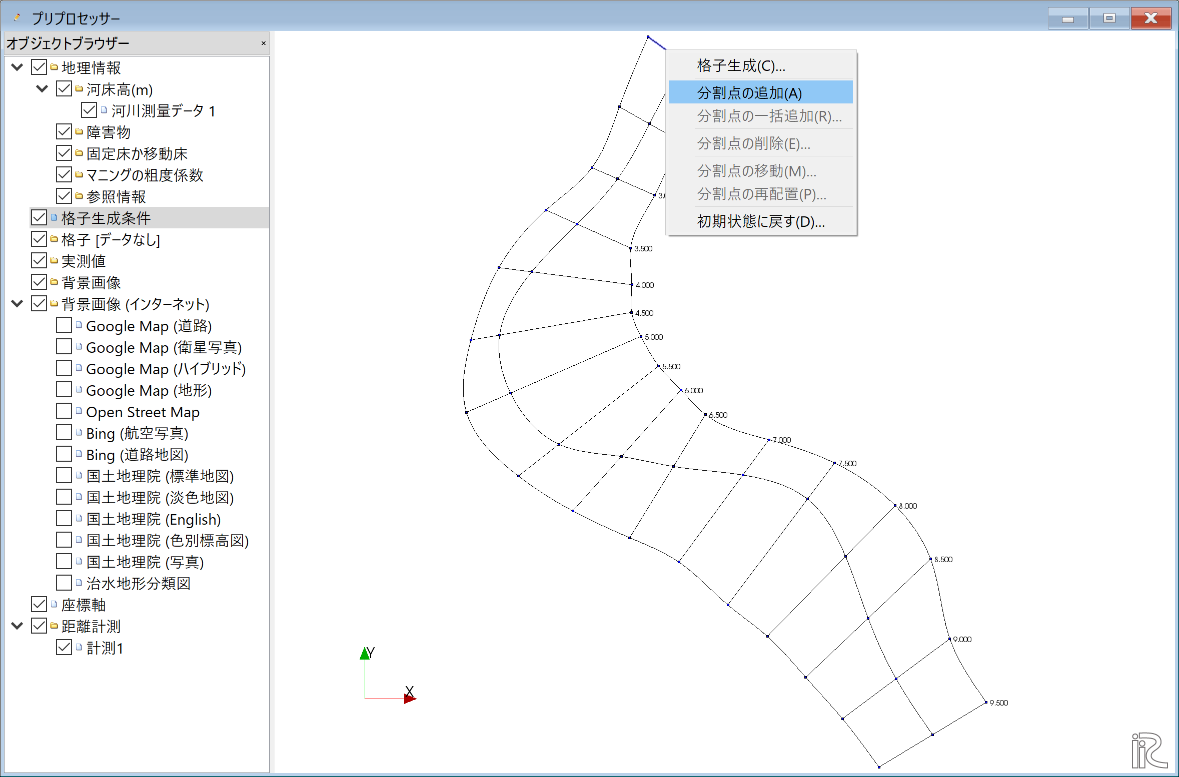
Figure 132 :分割点の追加(1)
「分割数」ここでは[8](中央から半分の断面を8分割するという意味)を指定して[OK]をクリック.
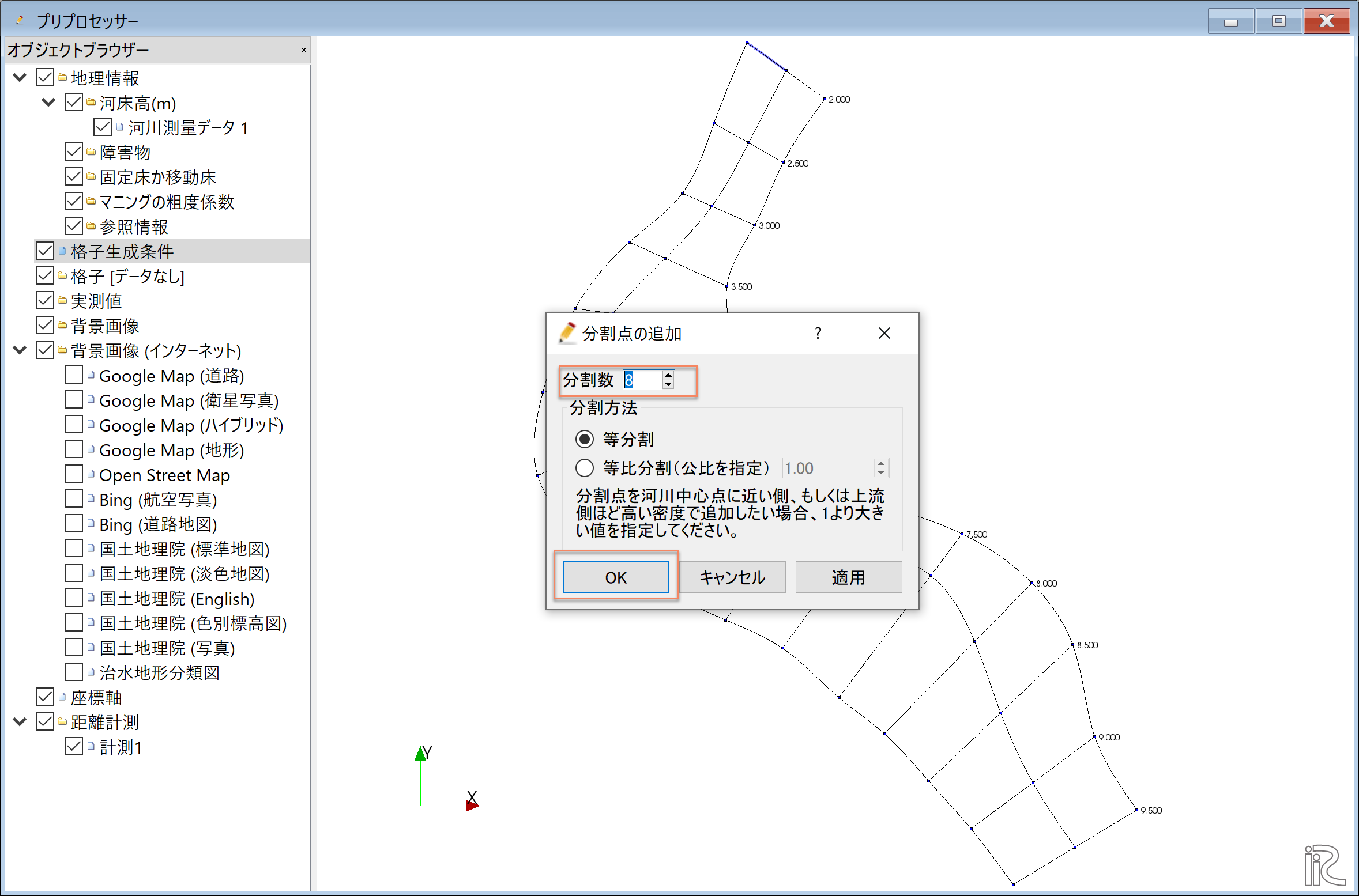
Figure 133 :分割点の追加(2)
Figure 132 で選択したのと反対側の横断線を選んで,右クリックし, 「分割点の追加(A)」を選択する.
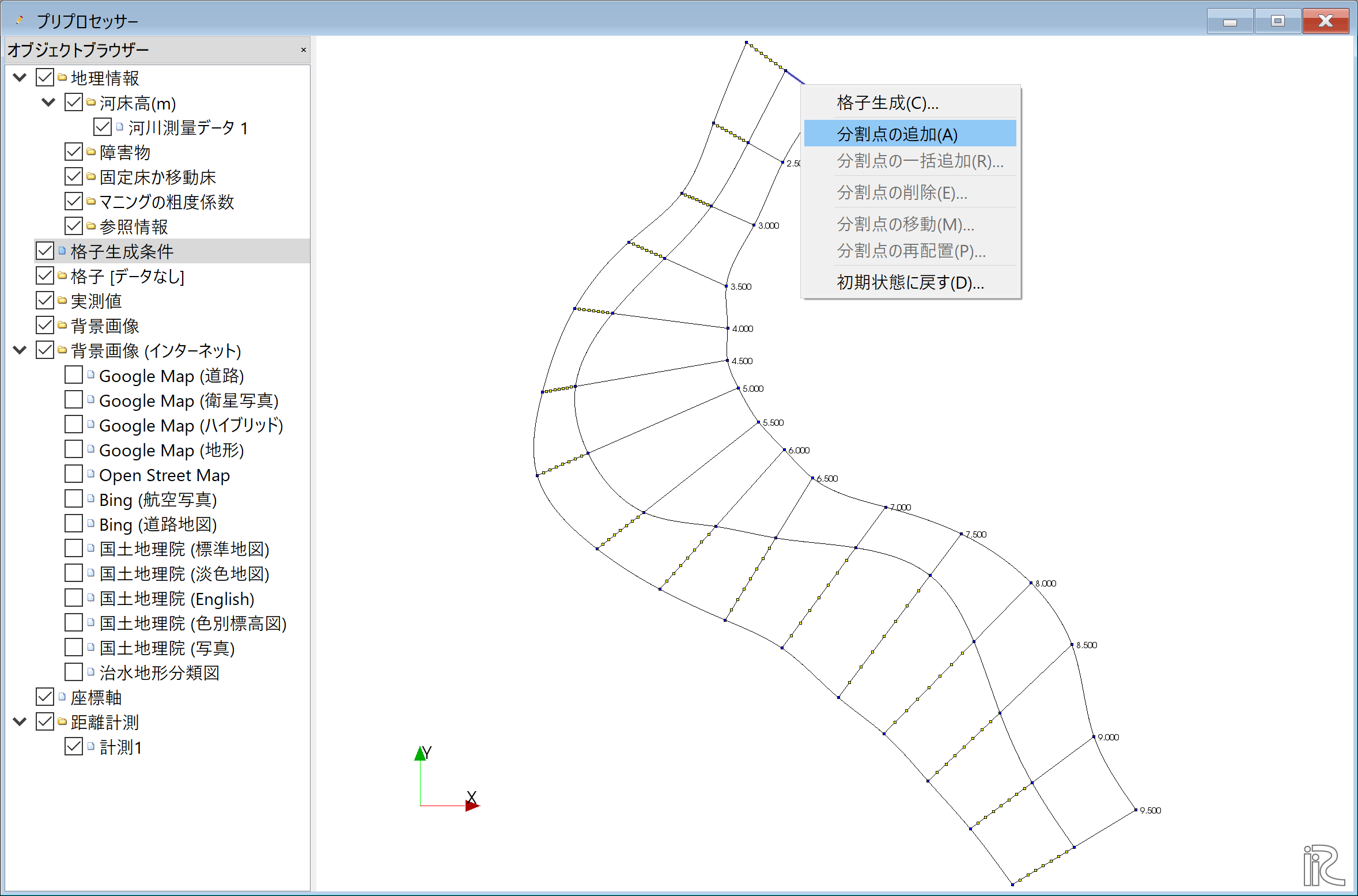
Figure 134 :分割点の追加(3)
「分割数」ここでは[4] Figure 133 で指定したのと同じく 左右岸対称の分割数とする.
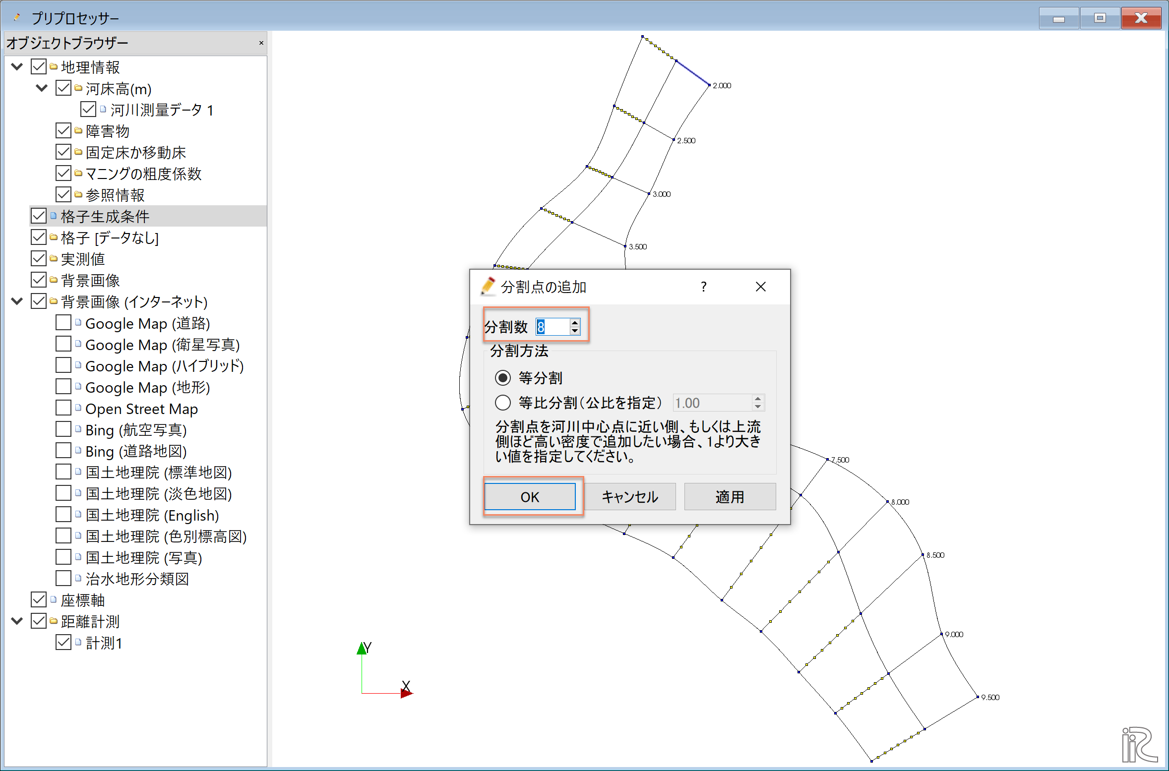
Figure 135 :分割点の追加(4)
縦断方向の分割数は一括して指定する.メニューバーから「格子」「格子生成条件」 「分割点の一括追加」を選択
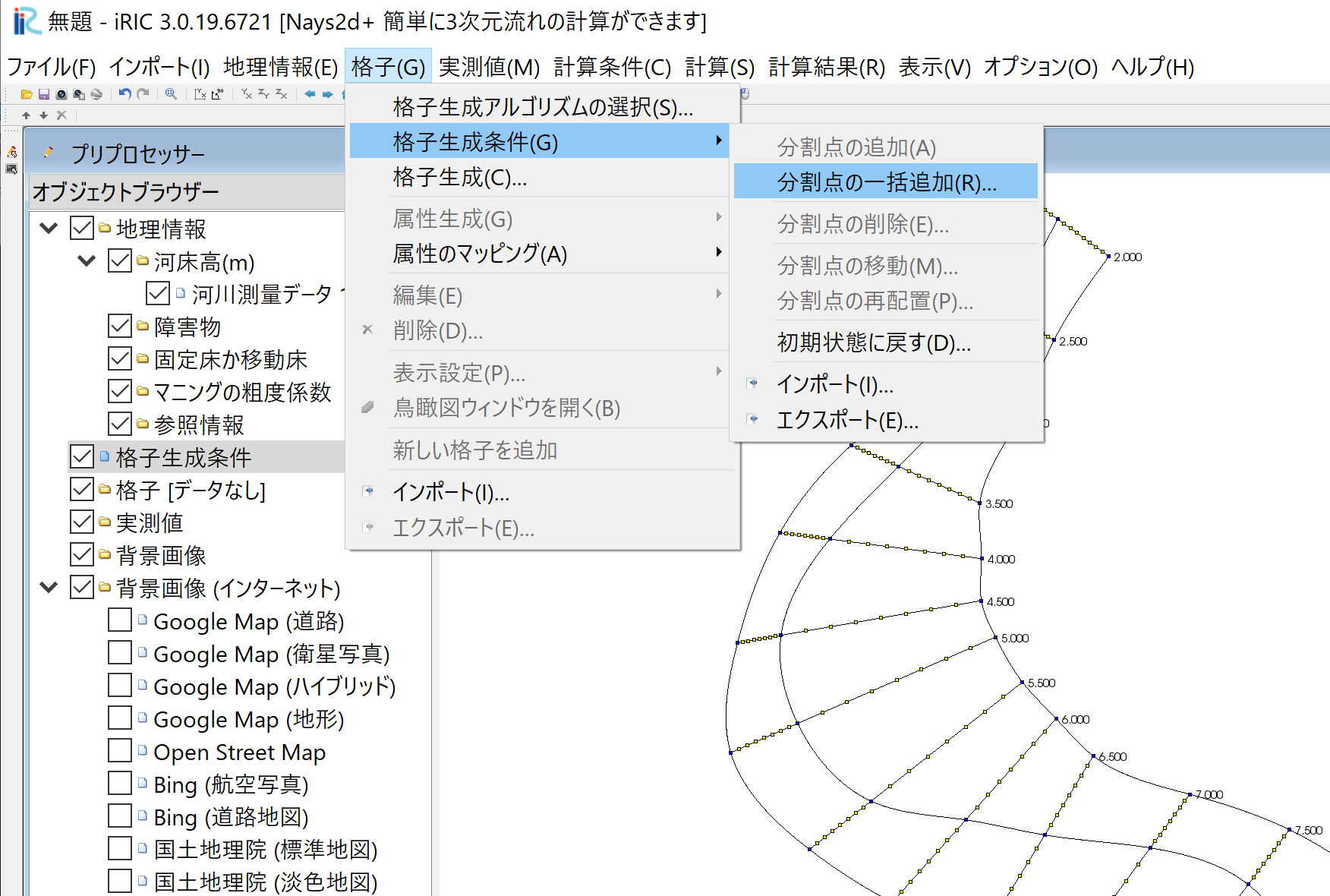
Figure 136 :分割点の一括追加(1)
「目標とする分割点間の距離」を選び,ここでは[50]mを指定して,[OK]をクリック.
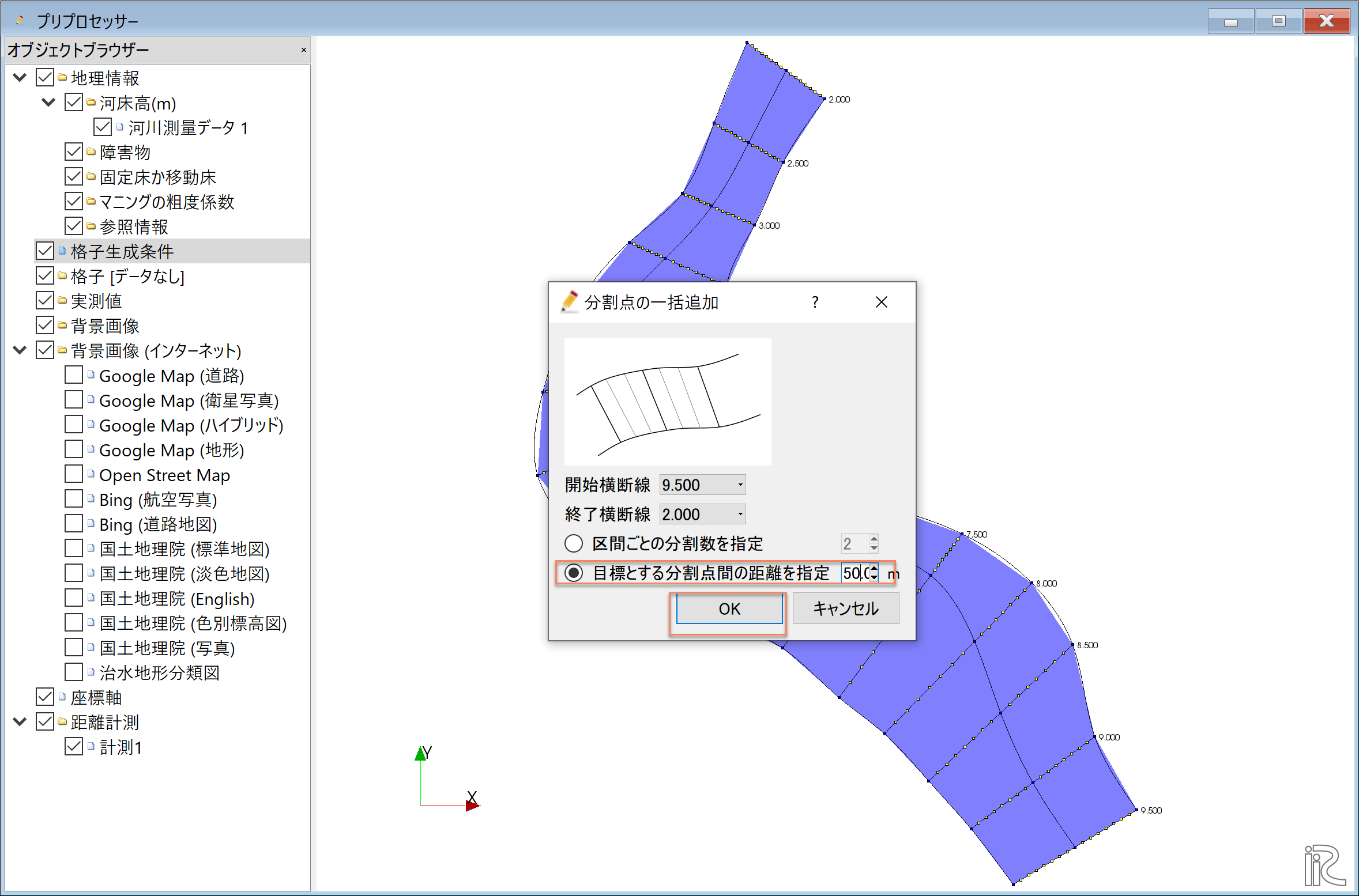
Figure 137 :分割点の一括追加(2)
分割点の設定が完了.縦横断方向の分割点に黄色の〇が付いた平面図が表示される.
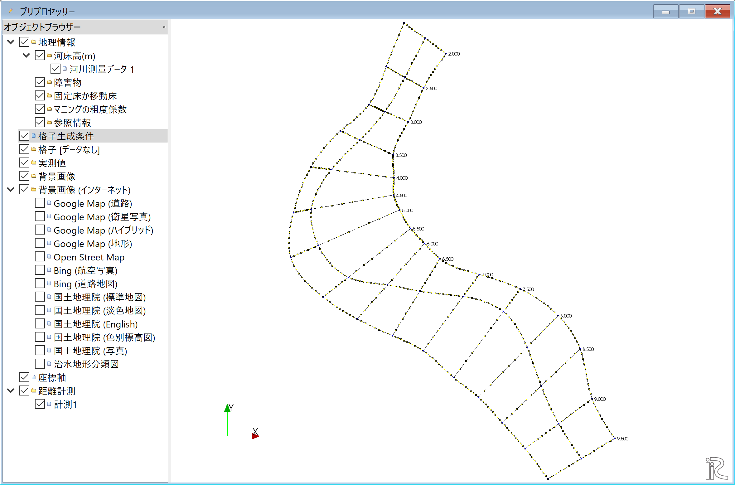
Figure 138 :分割点の設定完了
メニューバーの「格子」「格子生成」を選ぶ.
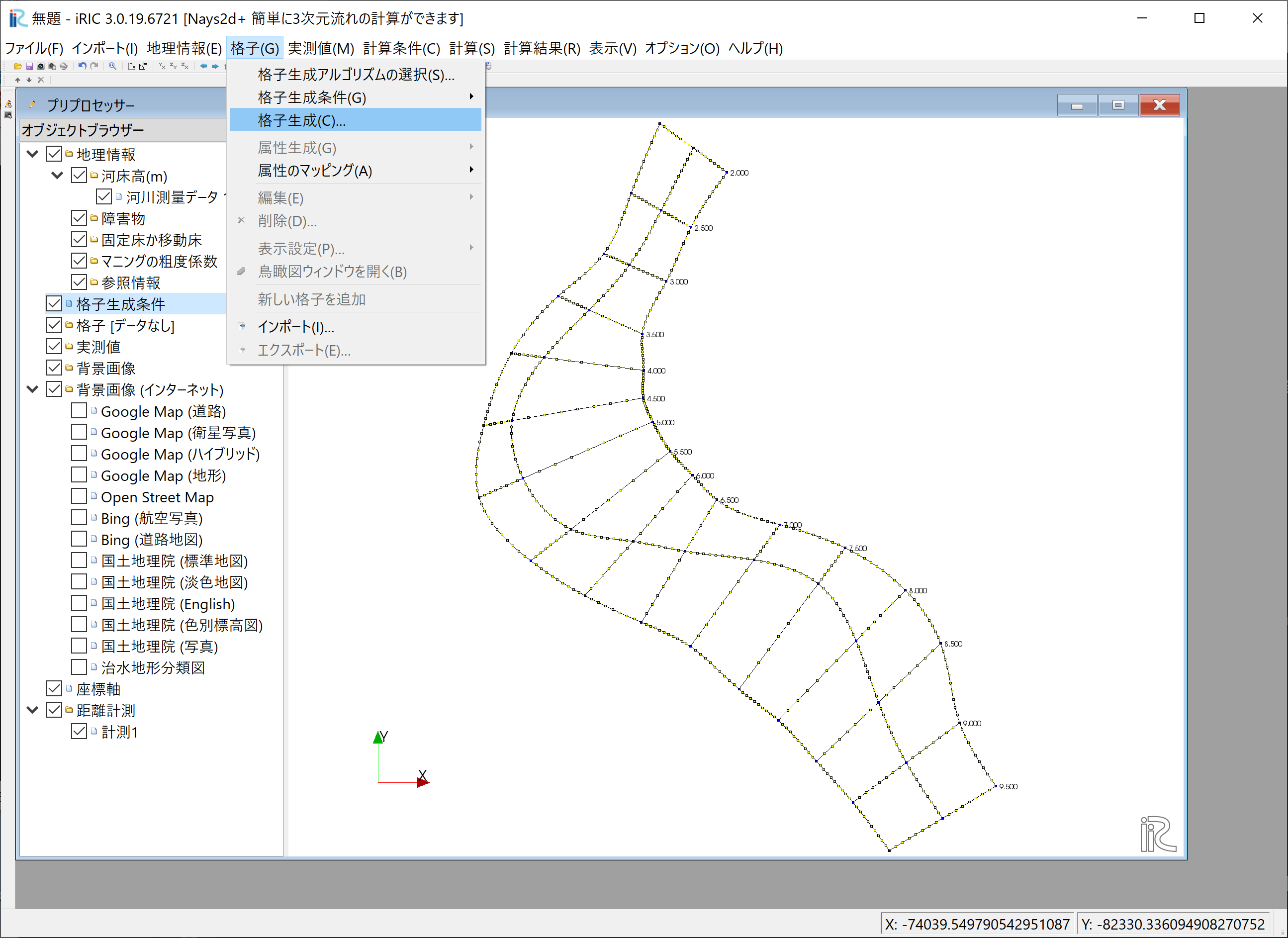
Figure 139 :格子生成(1)
格子生成範囲が青で塗られて,範囲の距離標を示すウィンドウが現れるので,確認して [OK]をクリックする.
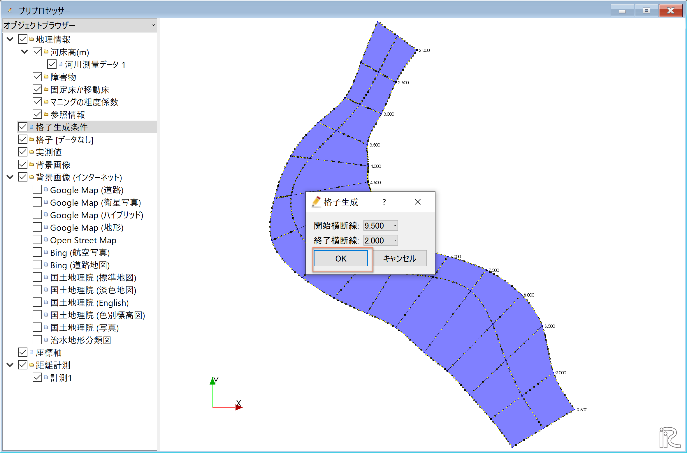
Figure 140 :格子生成(2)
「マッピングを実行しますか?」と出るので[OK]をクリックする.
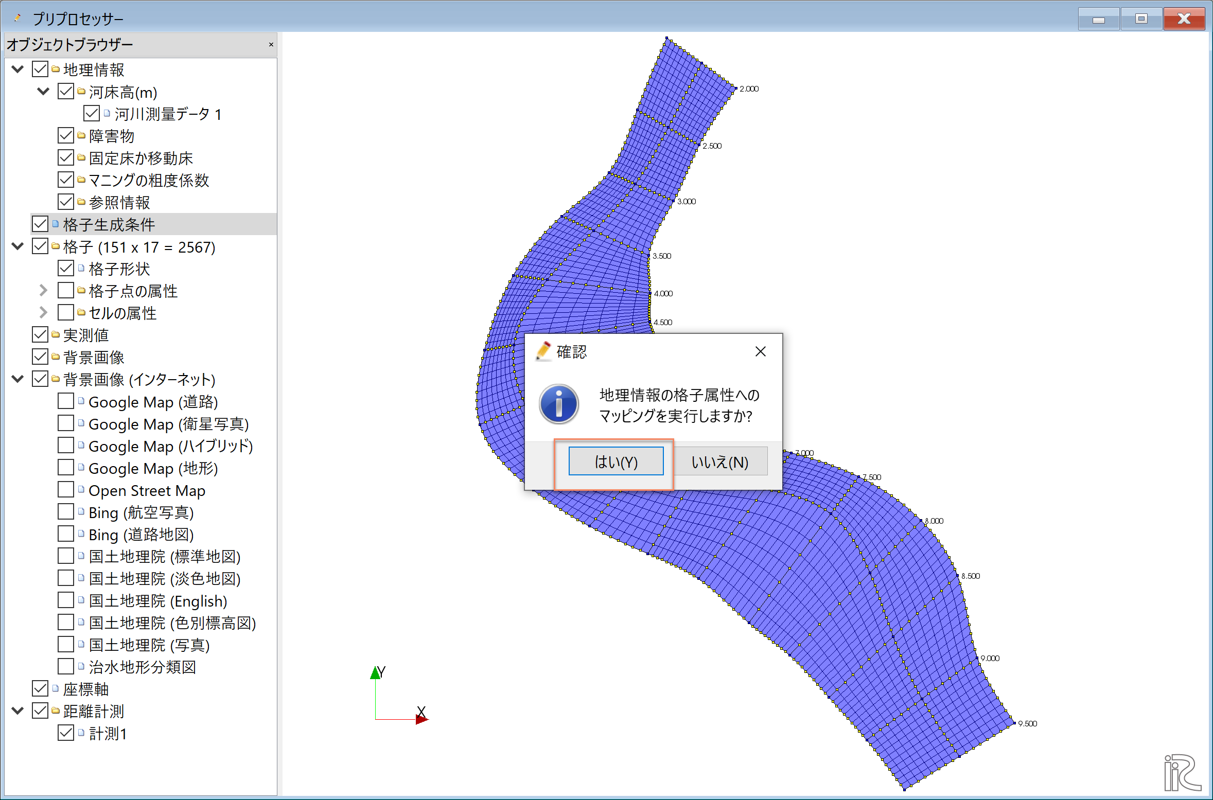
Figure 141 :マッピングの実行確認
格子生成が完了し,格子が表示される.
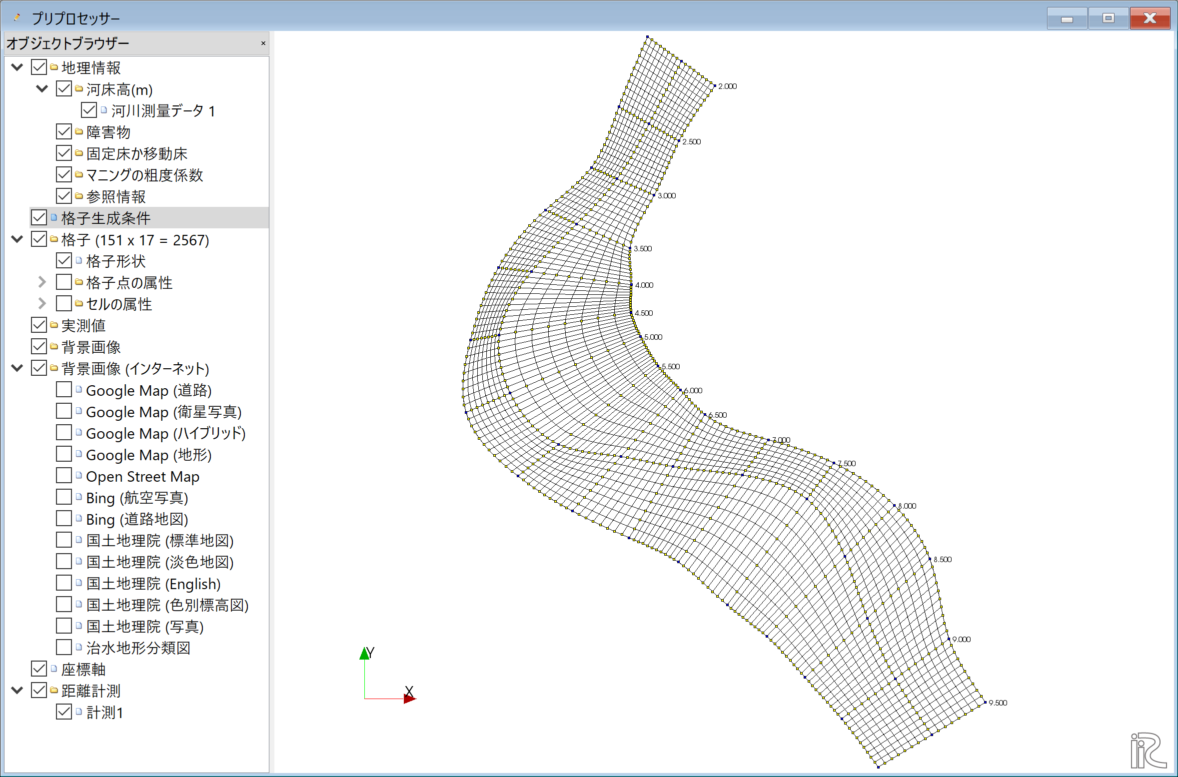
Figure 142 :格子生成の完了
オブジェクトブラウザーの「格子」「格子点の属性」「河床高(m)」に☑マークを入ると, 格子平面図に標高がカラーコンターで表示され,マッピングの結果が確認出来る.
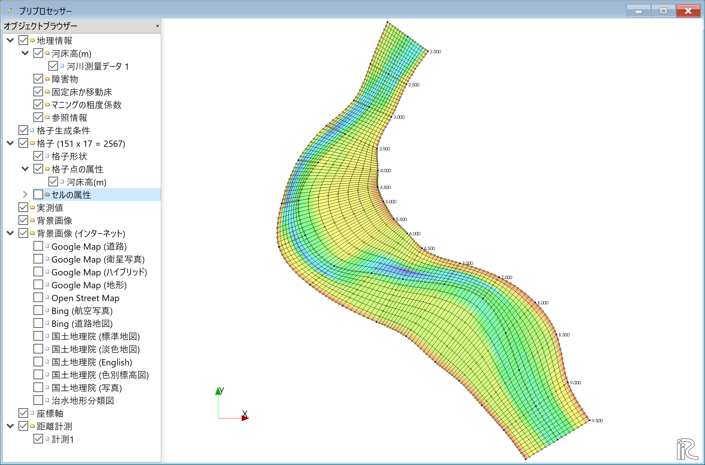
Figure 143 :マッピング結果の確認
計算条件の設定
メニューの「計算条件」「設定」を選ぶ
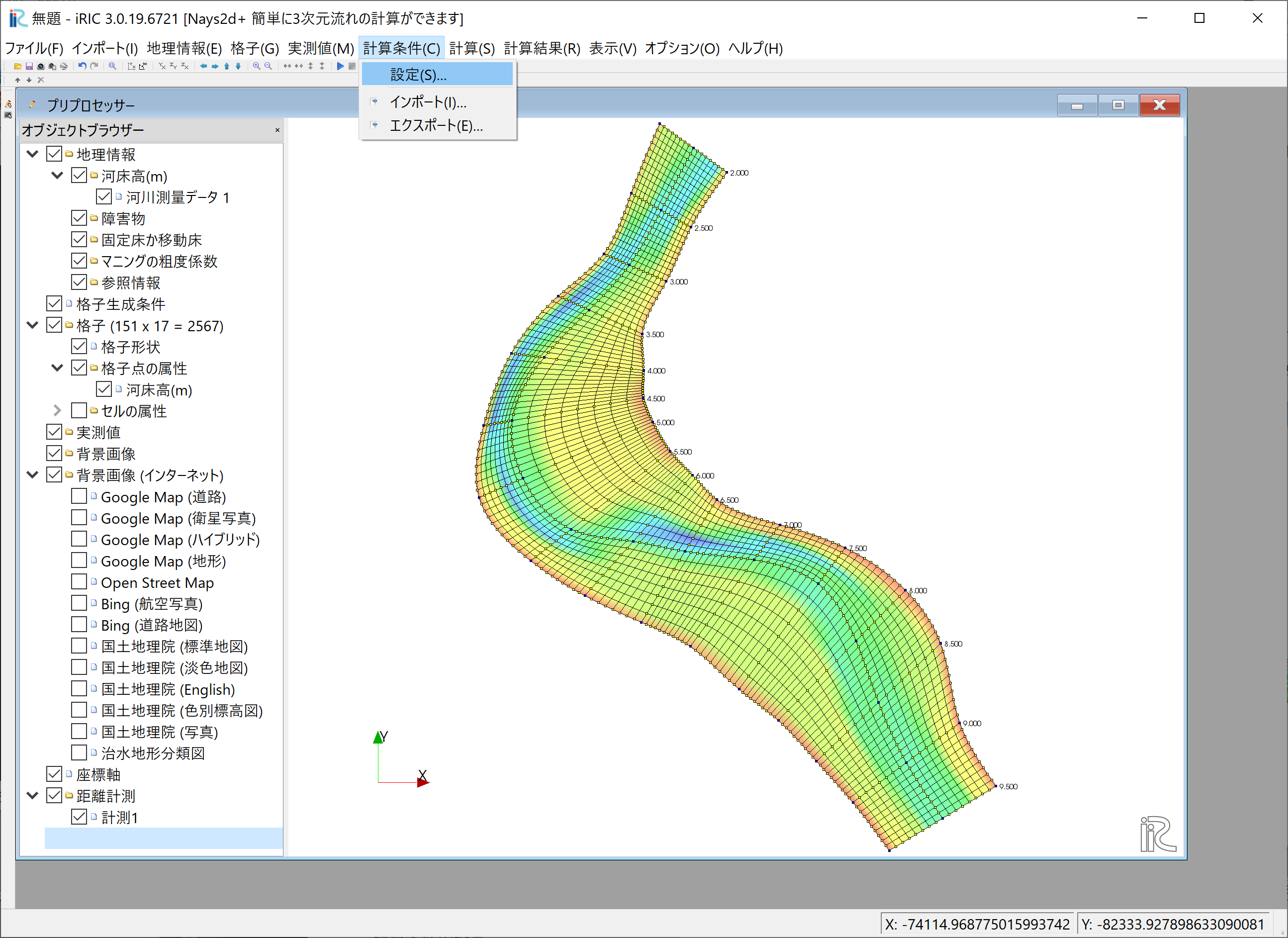
Figure 144 :計算条件の設定
「グループ」「流量および下流端水位の設定」で,「流量を与える時間単位」を[時間]とし, [Edit]をクリックする.
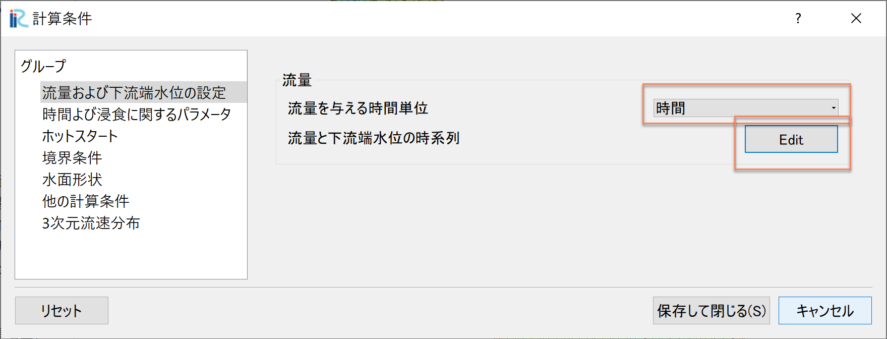
Figure 145 :流量の設定(1)
Figure 146 で3時間の一定流量[2,000㎥/s]を設定して[OK]をクリックする.
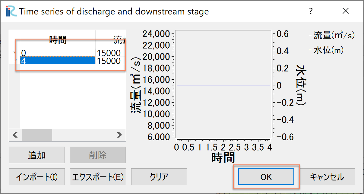
Figure 146 :流量の設定(2)
「時間および浸食に関するパラメーター」は下図ように設定する.
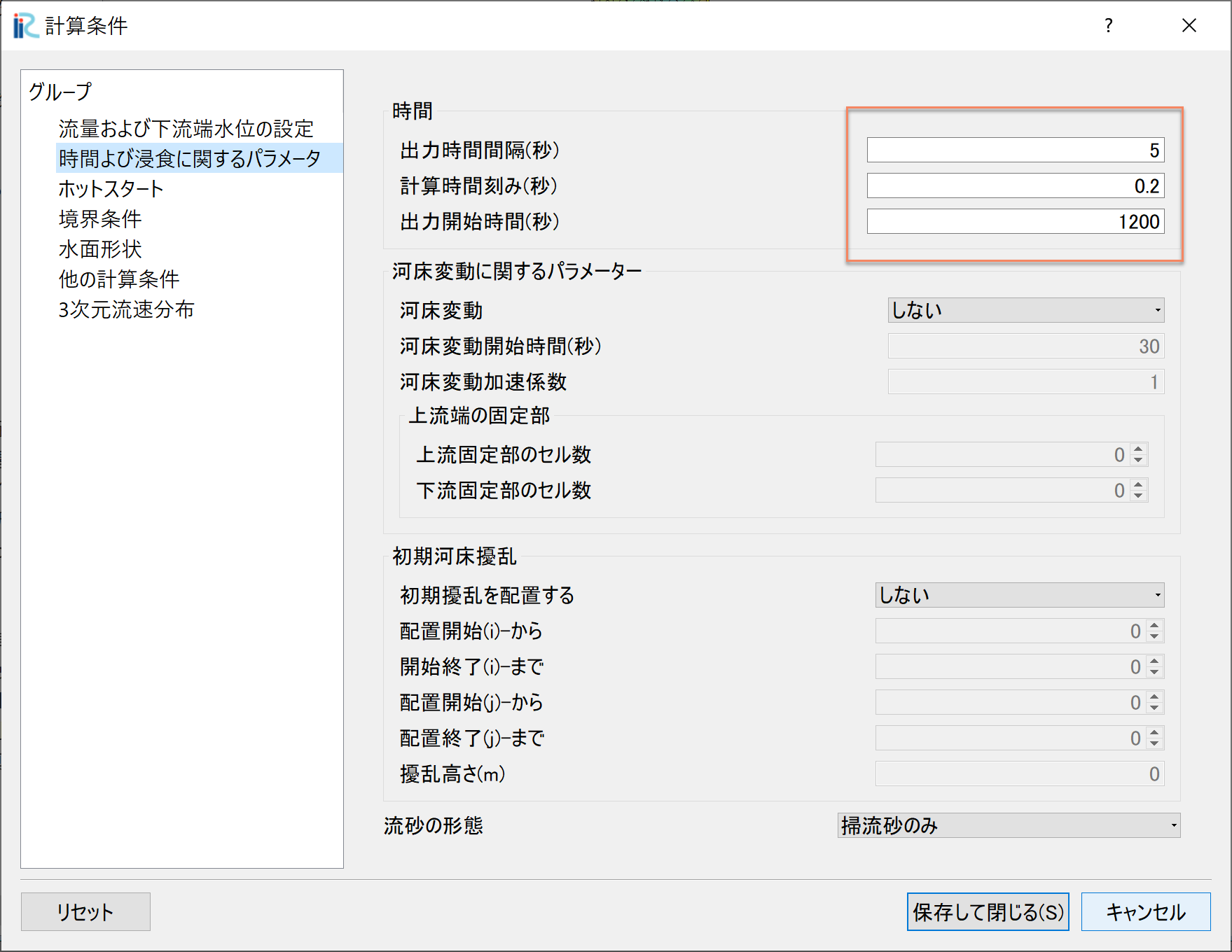
Figure 147 :時間および浸食に関するパラメーター
「3次元流速分布」に関しては下図のように設定して.[保存して閉じる]を選択して終了
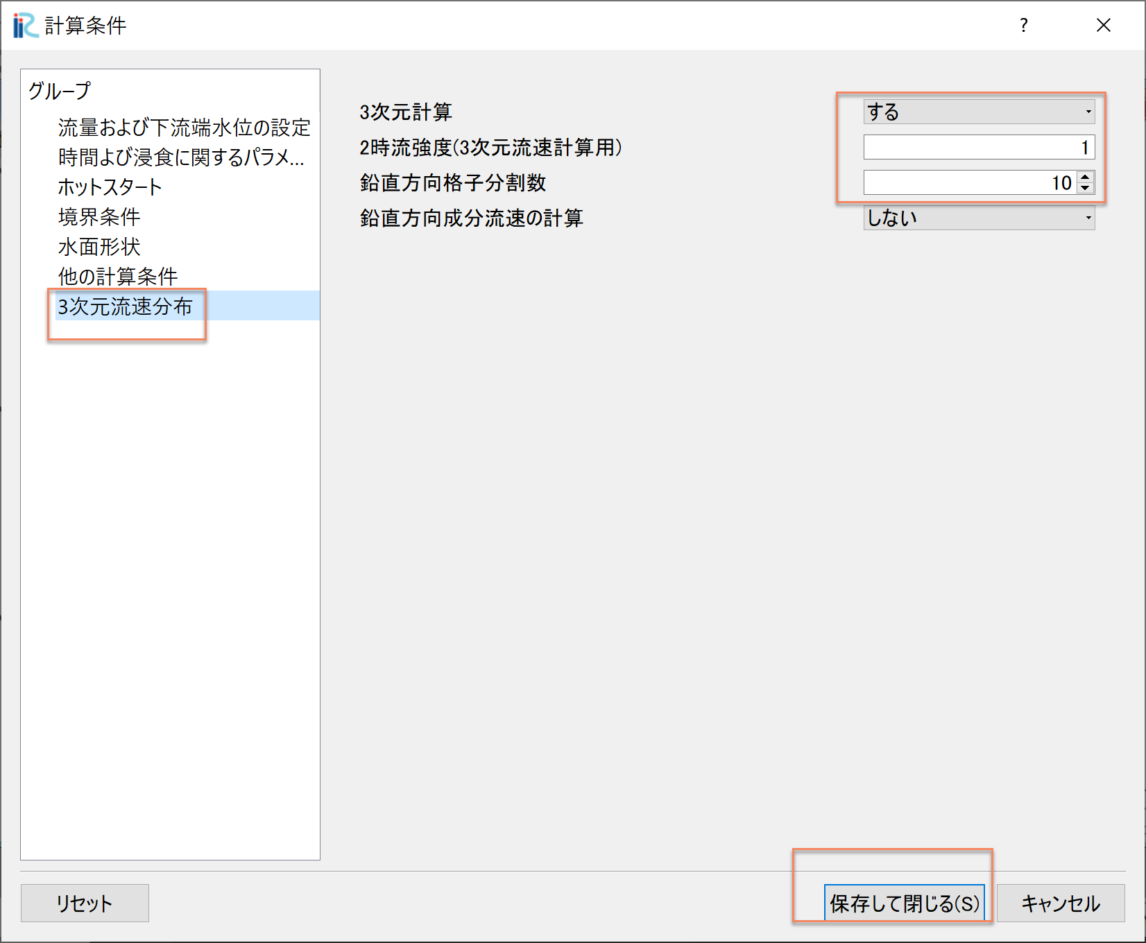
Figure 148 :3次元流速分布の設定
計算の実行
メニューバーで,「計算」「実行」を選択

Figure 149 :計算の実行(1)
「プロジェクトを保存しますか?」と聞かれるので,「はい(Y)」を選んで,適当な名前で 保存すると計算が開始される.
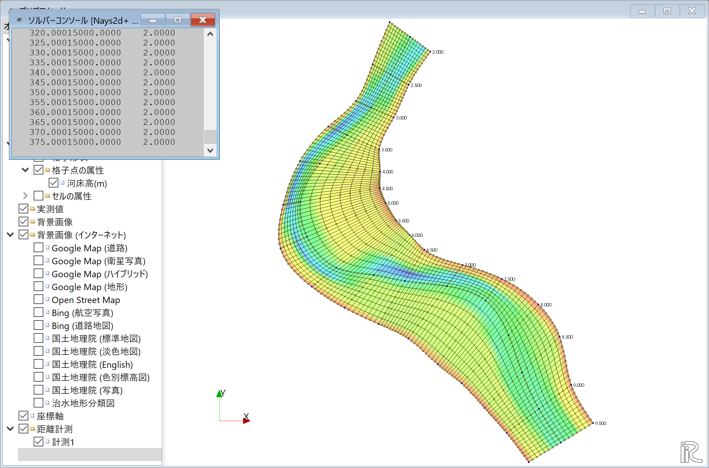
Figure 150 :計算の実行(3)
「計算が終了しました.」と出るので,[OK]をクリックする.
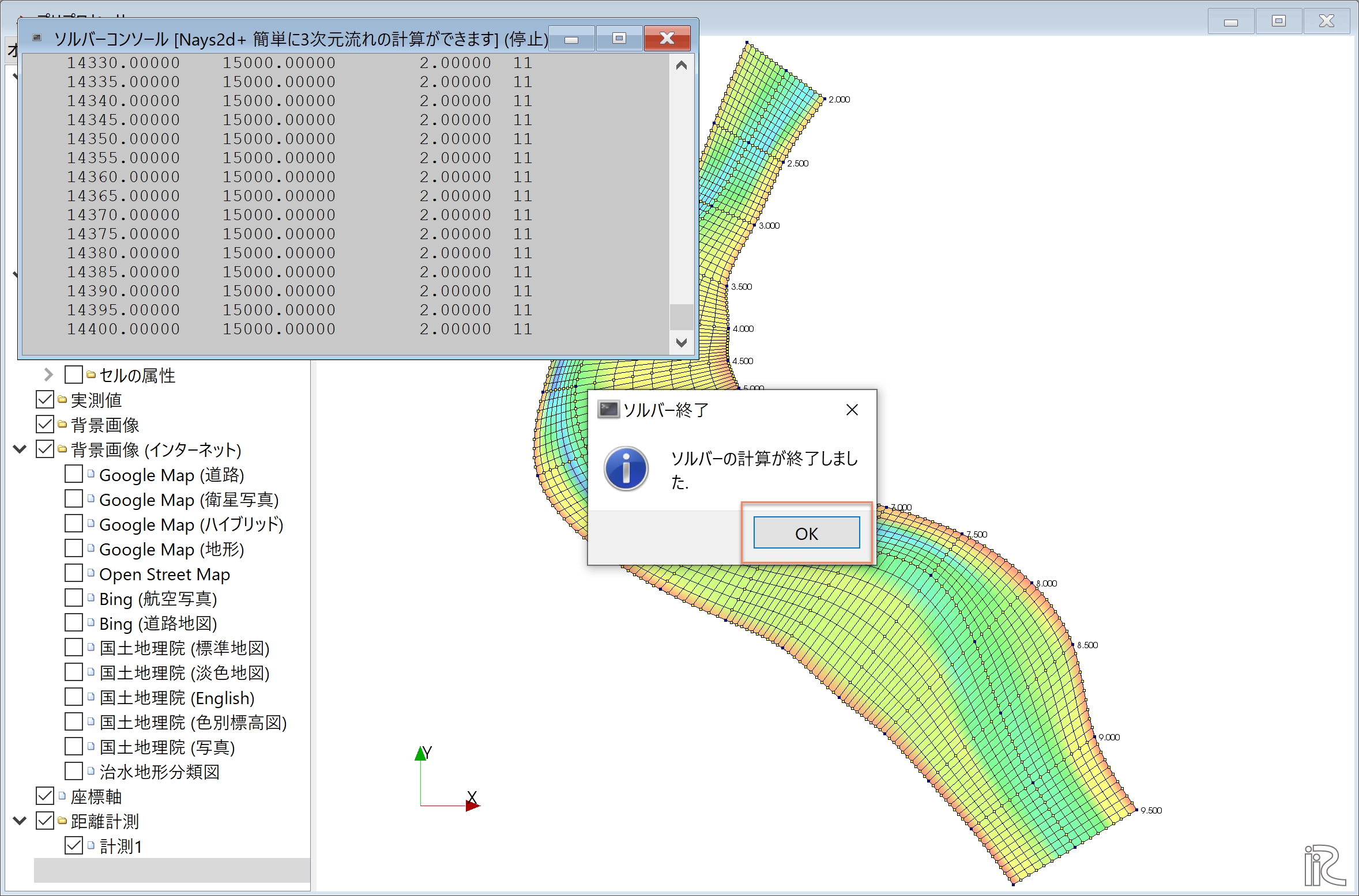
Figure 151 :計算の終了
計算結果の表示
メニューで「計算結果」「新しい可視化ウィンドウ(2D)を開く」を選択する.
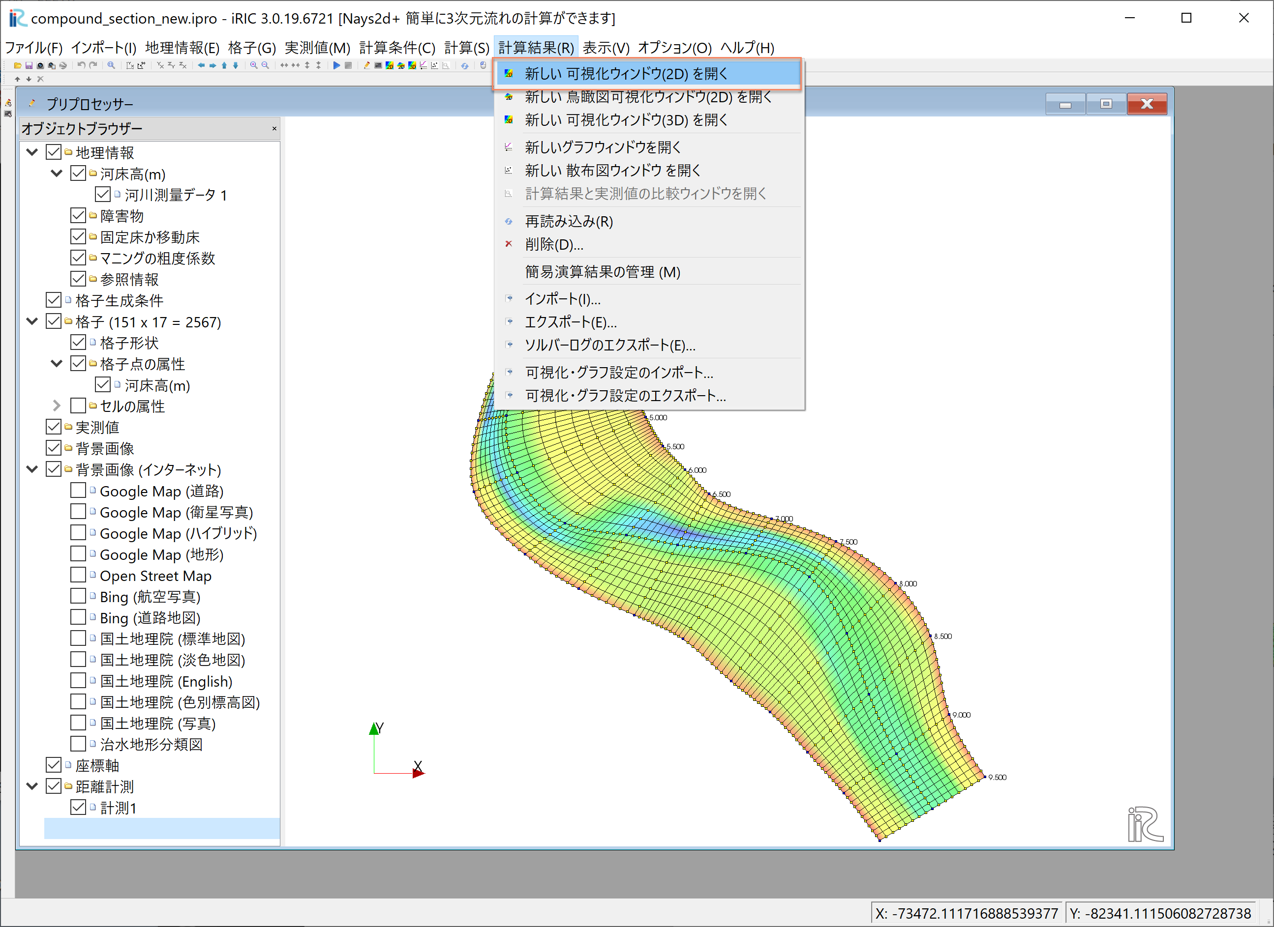
Figure 152 :新しい可視化ウィンドウ(2D)を開く
可視化ウィンドウが表示されるので,サイズを適当に変更して見やすい状態にする.
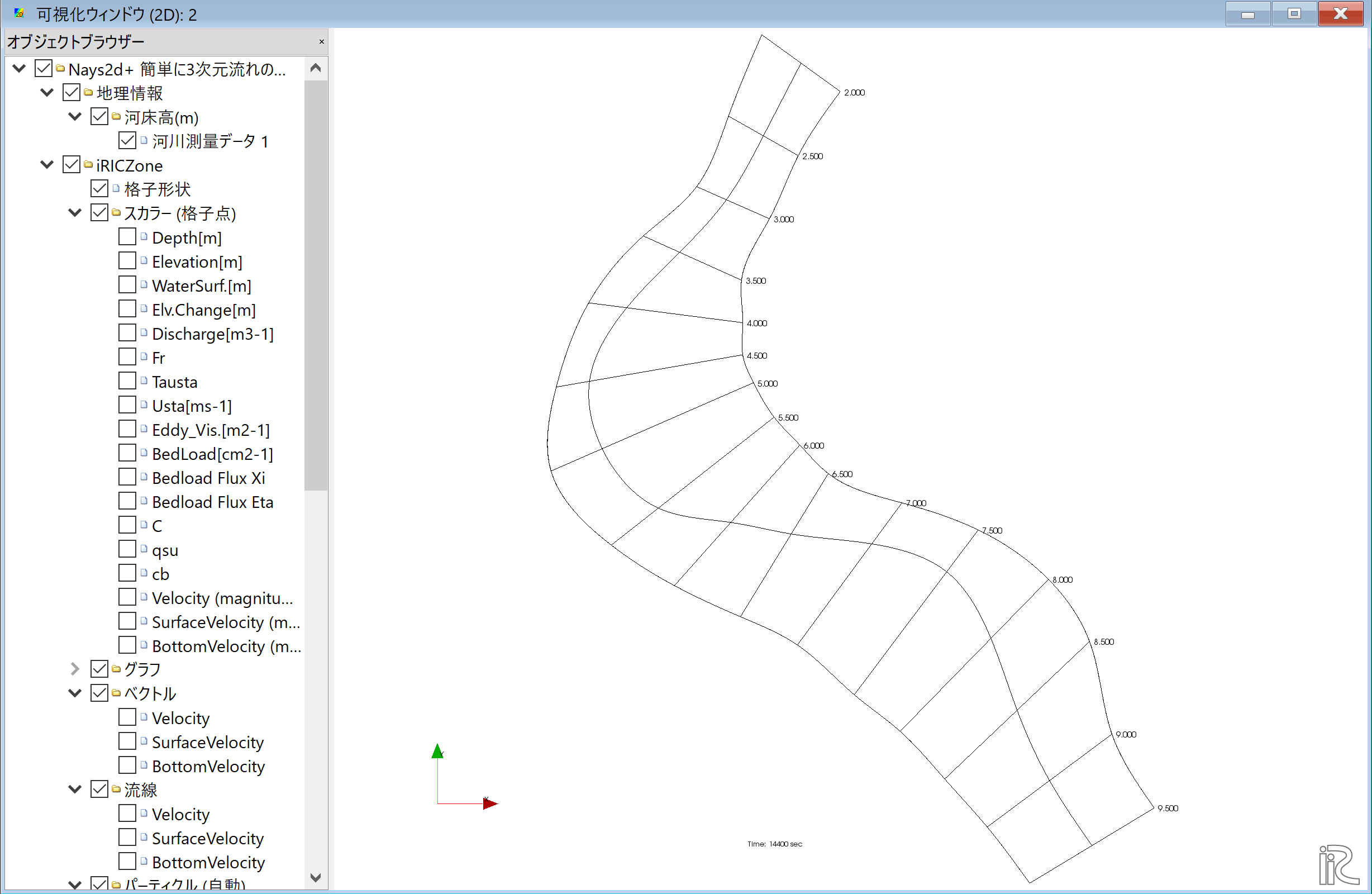
Figure 153 :新しい可視化ウィンドウ(2D)の表示
水深の表示
Figure 154 のように.オブジェクトブラウザーで, 「スカラー(格子点)」「Depth(m)」 に☑マークを入れて,[Depth(m)]を右クリックで「プロパティ」を選択すると, 「スカラー設定ウィンドウ」 Figure 155 が表示される.
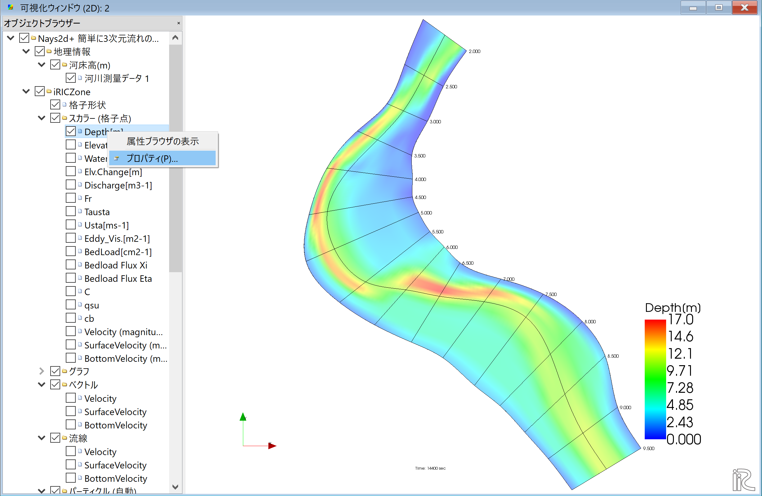
Figure 154 :新しい可視化ウィンドウ(2D)の表示
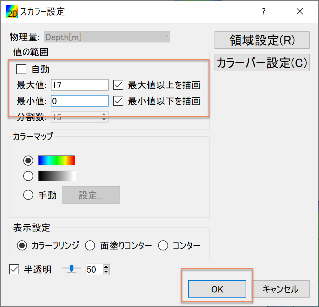
Figure 155 :スカラー設定
「スカラー設定ウィンドウ」 Figure 156 を図のように設定して[OK]をクリックすると, 水深コンターが表示される.
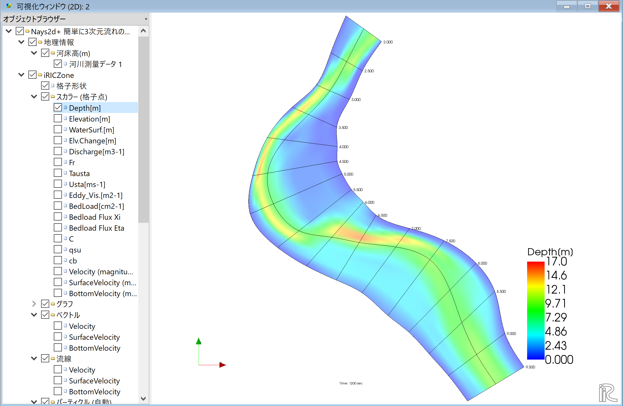
Figure 156 :水深コンター図
背景画像の表示
「ファイル」「プロパティ」を選択する.
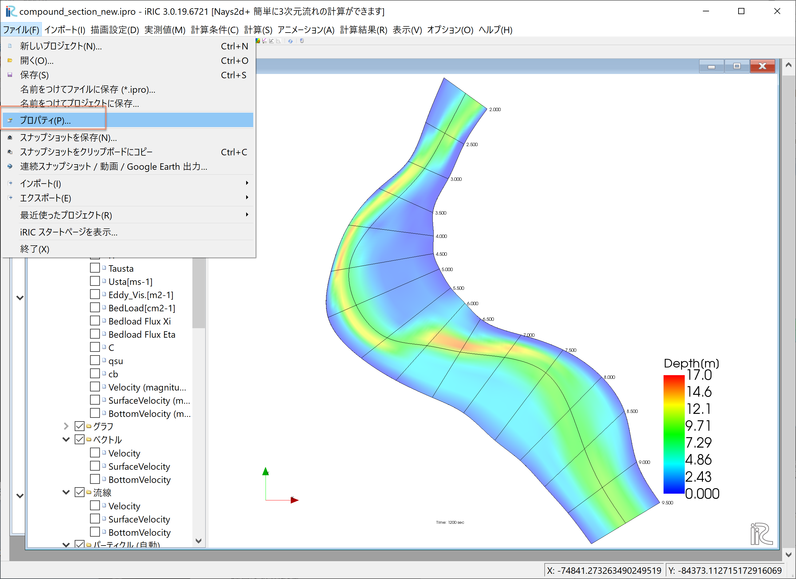
Figure 157 :ファイルのプロパティ選択
「プロジェクトプロパティ」で「座標系」の「編集」を選択する.
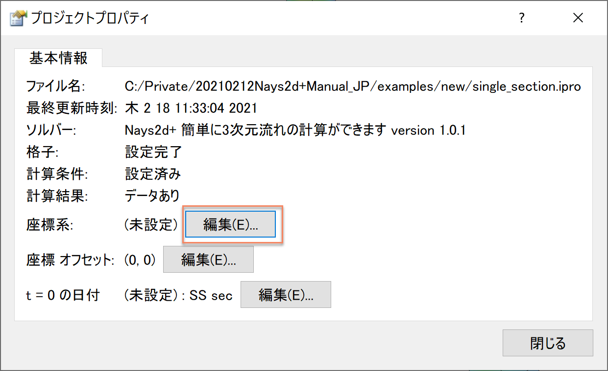
Figure 158 :座標系の編集
「座標系の選択」画面で,「検索」に[Japan]と入れると,「EPSG.......」というのが沢山出てくるので, その中で,末尾が「XII」のものを選んで[OK]をクリックする. (日本の座標系については, http://www.gsi.go.jp/sokuchikijun/jpc.html を参照されたい.)
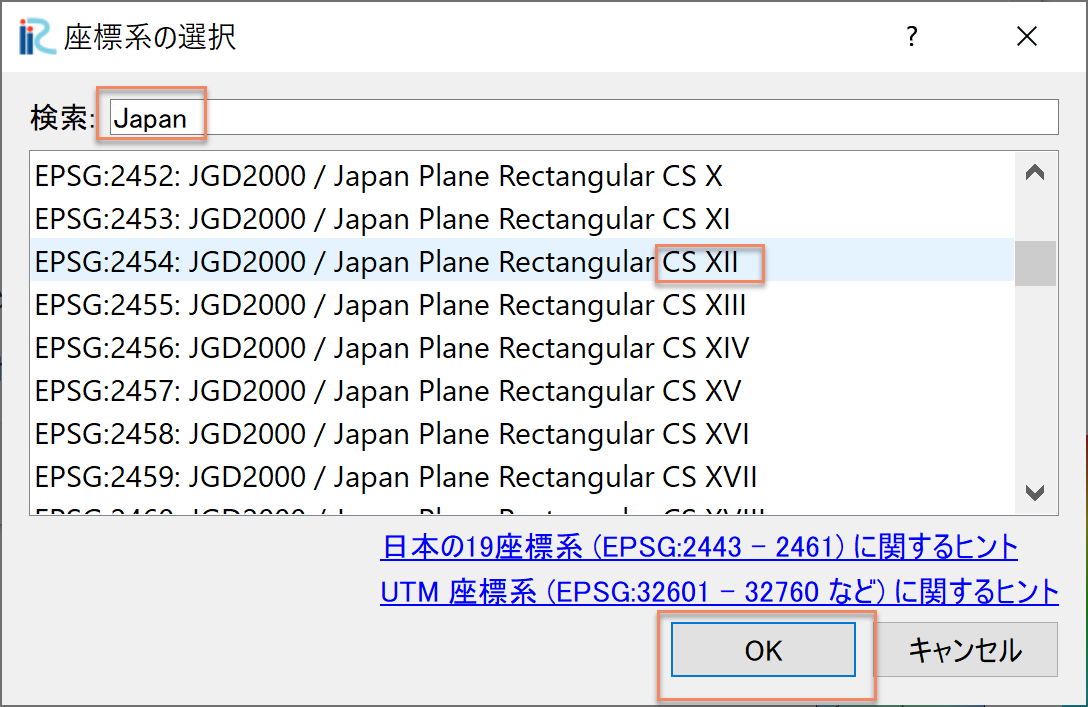
Figure 159 :座標系の選択
「プロジェクトプロパティ」ウィンドウを[閉じる]
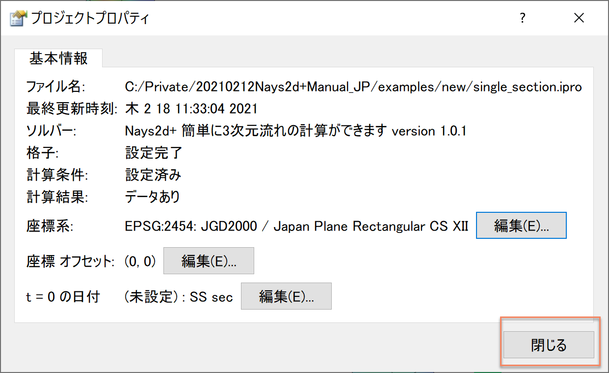
Figure 160 :プロジェクトプロパティウィンドウを閉じる
オブジェクトブラウザーで,「背景画像(インターネット)」「国土地理院(標準地図)」 に☑マークを入れると,背景地図が読み込まれ,表示される.
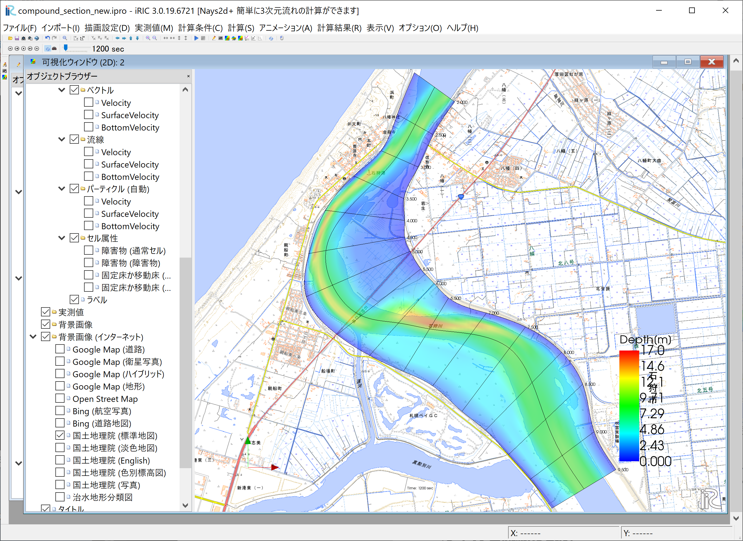
Figure 161 :背景画像の読み込み完了
背景を写真にしたい場合や,他の種類の地図にしたい場合は,別の項目を☑する. なお,GUIの操作時に常時背景画像を表示させておくと,操作が非常に重くなるので, 通常は「背景画像」の☑マークを外しておくことを推奨する.
ベクトルと流線の表示
操作方法,表示方法は全章の例と全く同じなので,省略する.
パーティクルアニメーションの表示
オブジェクトブラウザーの「パーティクル」「Velocity」に☑マークを付けて, タイムバーをゼロに戻し,プレイボタンを押す( Figure 162 )と Figure 163 の水深平均流速によるパーティクルアニメーションが始まる.
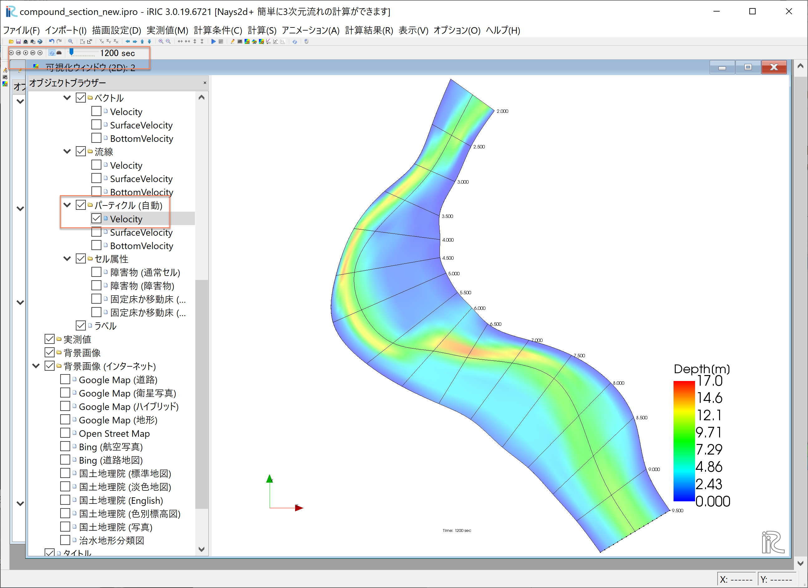
Figure 162 :パーティクルアニメーション

Figure 163 :水深平均流速によるパーティクル
表面流速に乗ったパーティクルを赤色で表示する. 「パーティクル」「SurfaceVelocity」に☑を入れて,「パーティクル」を右クリックして 「プロパティ」を選択すると,「パーティクル設定画面」 Figure 164 が表示されるので,図のように設定して[OK]をクリックする. タイムバーをゼロに戻して,プレイボタンを押すと Figure 165 の 表面流によるパーティクルアニメーションが表示される.
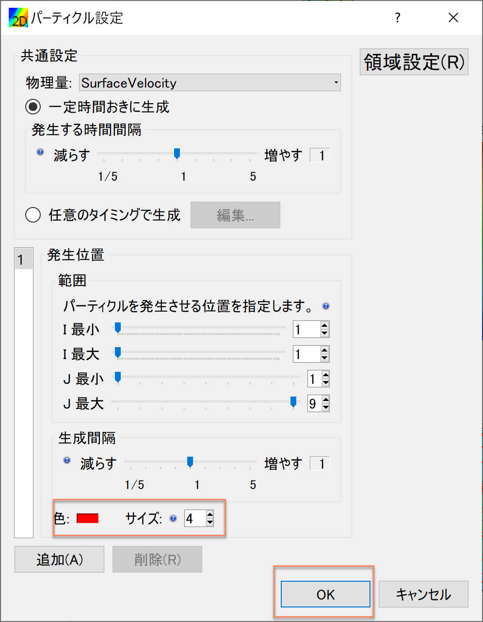
Figure 164 :パーティクル設定

Figure 165 :表面流速によるパーティクル
同様な手続きで,「BottomVelocity」を選択すると,底面流によるパーティクルを表示出来る.
Figure 166 :底面流速によるパーティクル