[Example 3] Flow in a Sine-Generated Curve Channel

Create Computational Grid

From the main menu, select [Grid], [Select Algorithm to Create Grid] ( Figure 55 )

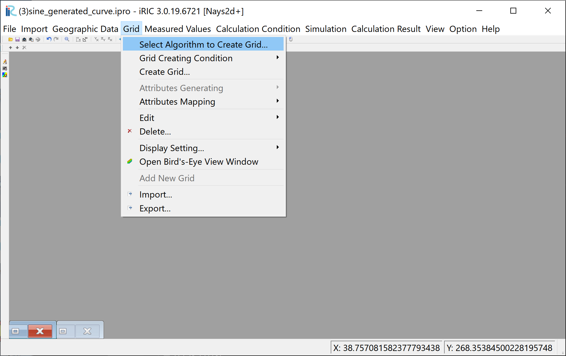
Figure 55 : Select Algorithm to Create Grid

Select [Simple Grid Generator] in Figure 56 , and click [OK].

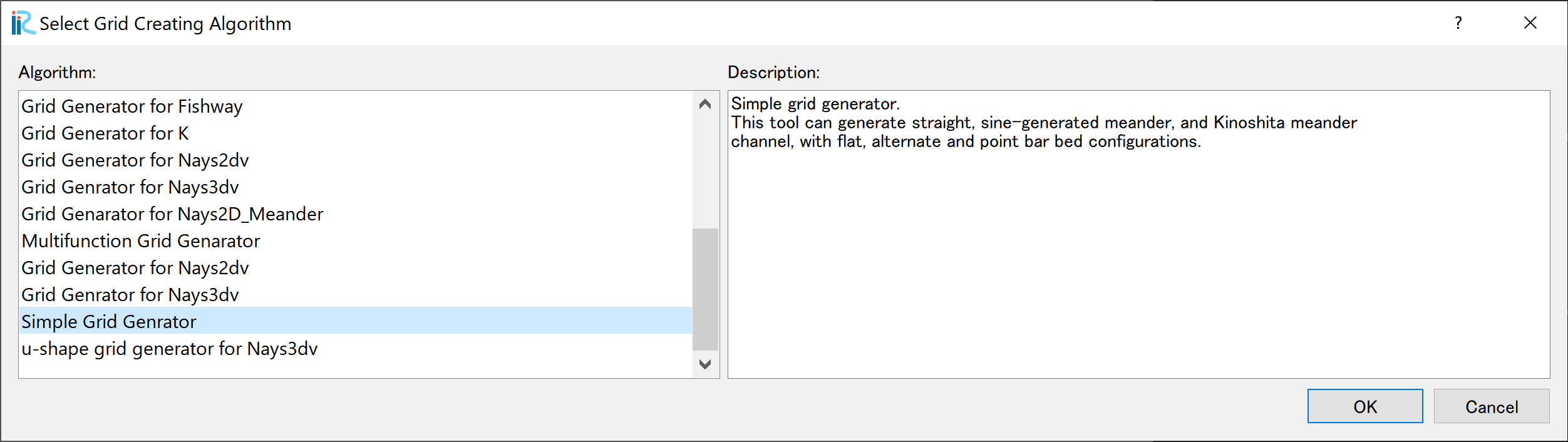
Figure 56 : Select Grid Creation Algorithm

Set “Channel Shape” values as Figure 57

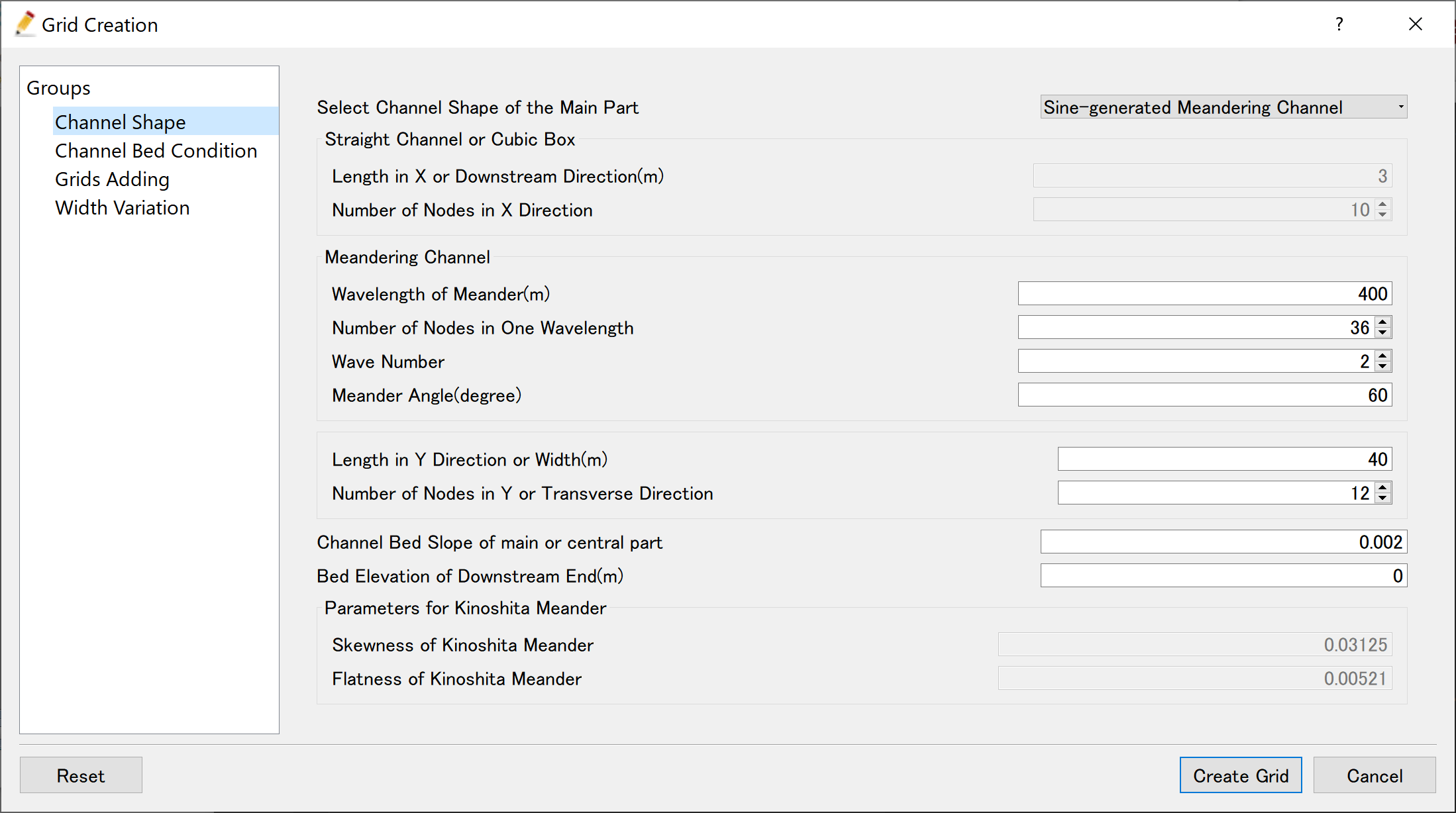
Figure 57 : Grid Creation: Channel Shape

Set “Channel Bed Condition” values as Figure 58 , and click [Create Grid]. Click [Yes(Y)] when you are asked “Figure 59 . Then the grid creation is completed.

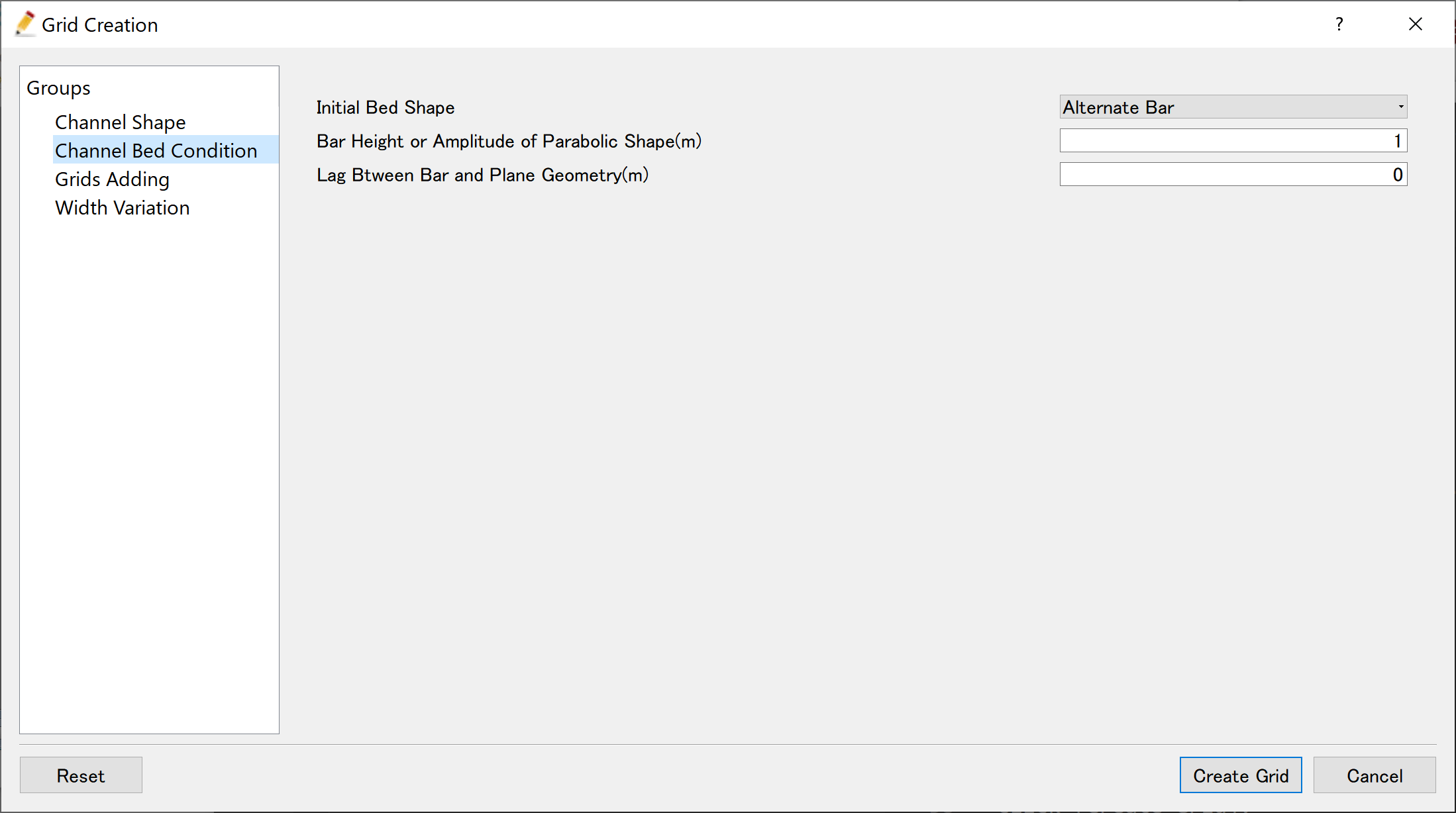
Figure 58 : Grid Creation: Channel Bed Condition

Figure 59 : Mapping？

Bed configuration and channel shape can be confirmed by putting checking marks at, [Grid], [Node attributes] and [Elevation (m)]. ( Figure 60 )

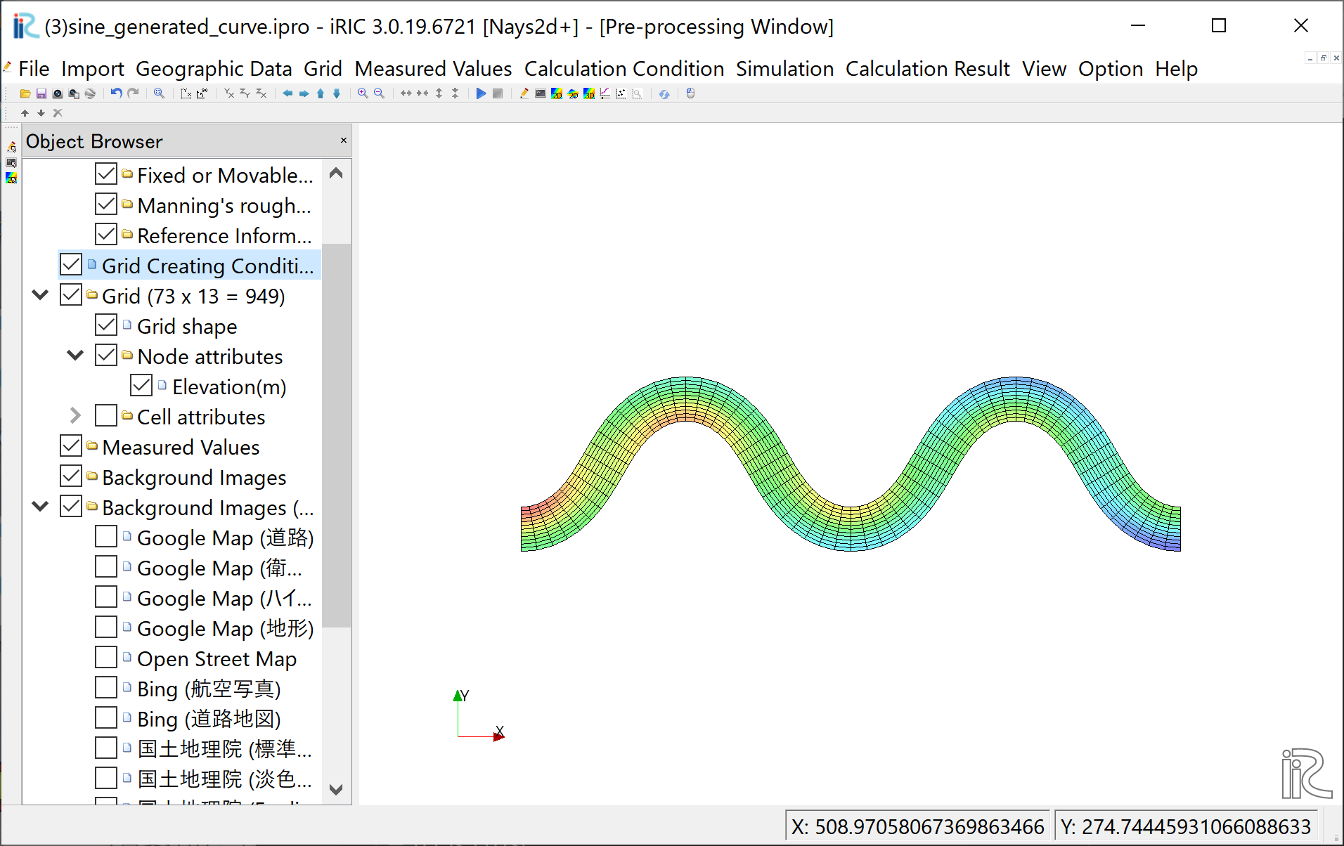
Figure 60 : Grid Creation Completed

Computational Condition

From the menu bar, select [Calculation Condition], [Settings] and [Calculation Condition] window, Figure 61 appears.

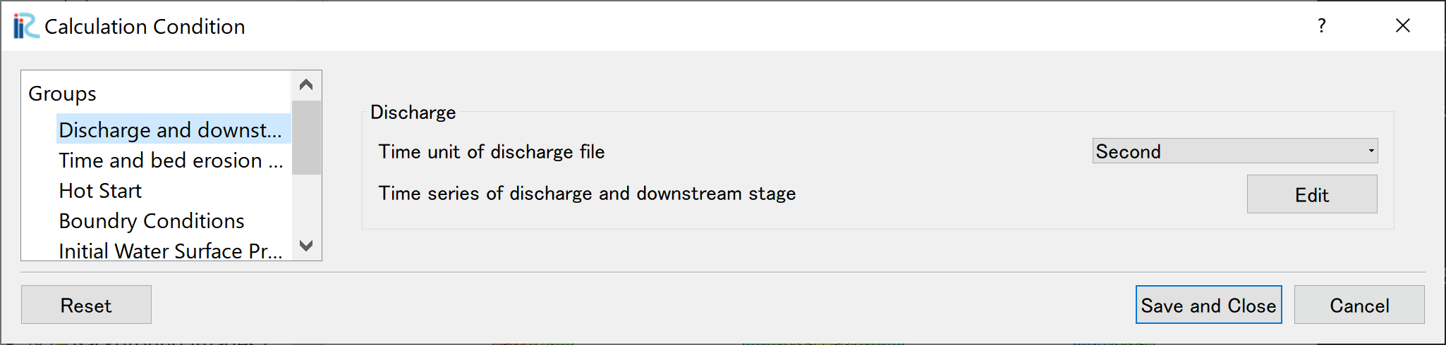
Figure 61 : Calculation Condition: Groups

In Figure 61 , select [Discharge and downstream water surface elevation] and click [Edit].

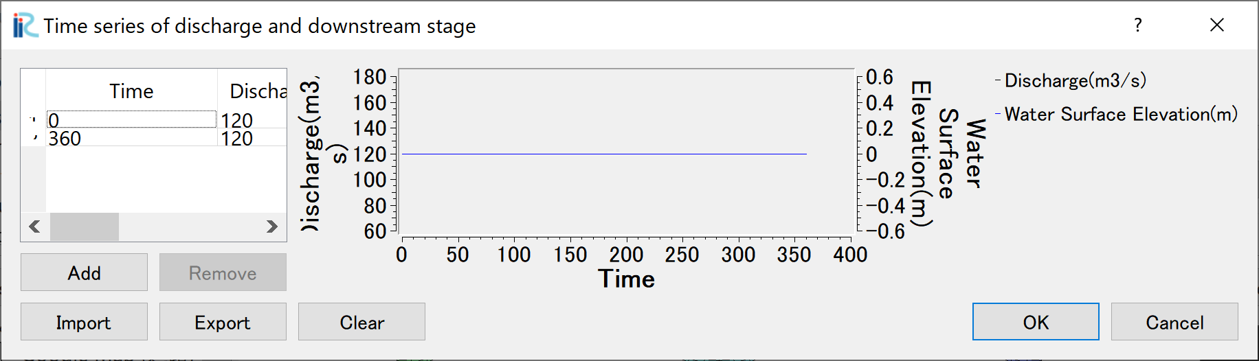
Figure 62 : Input discharge hydro graph

Input discharge hydrograph as shown in Figure 62 and click [OK].

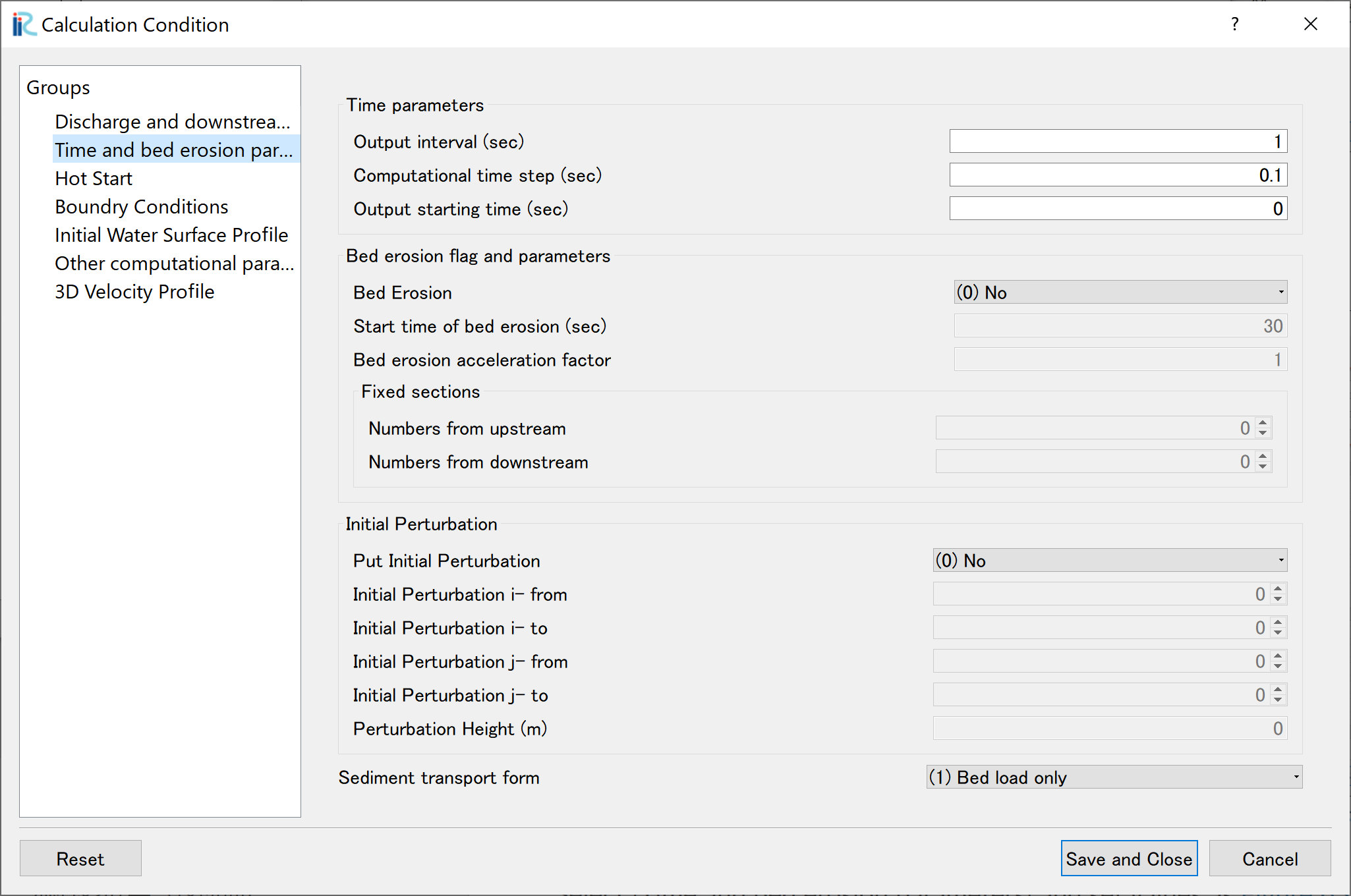
Figure 63 : Time and bed erosion parameters

Select [Time and bed erosion parameters] and set values as Figure 63 .

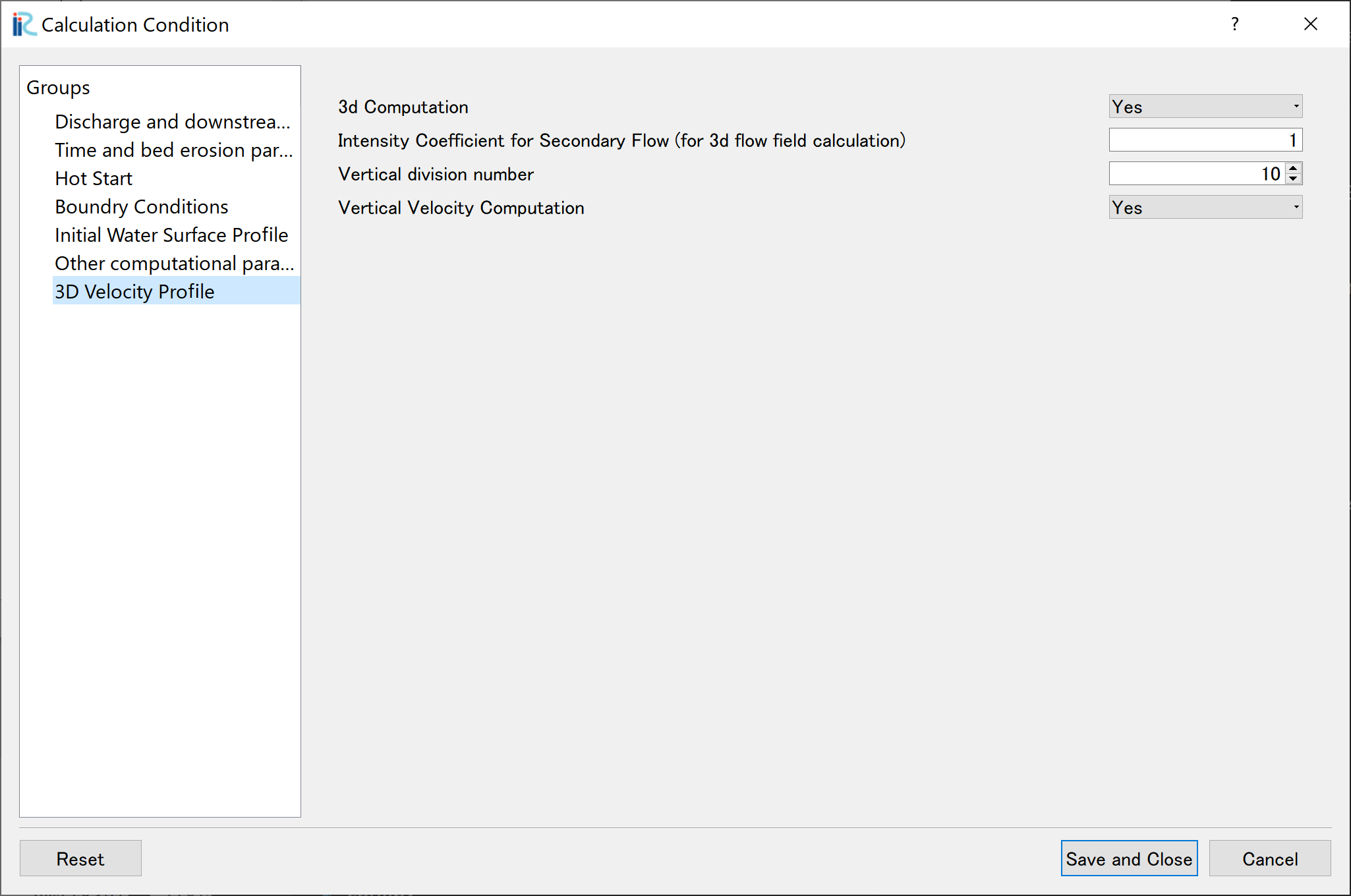
Figure 64 : 3D Velocity Profile

Set [3D Velocity Profile] as Figure 64, and click [Save and Close]

Launch Computation

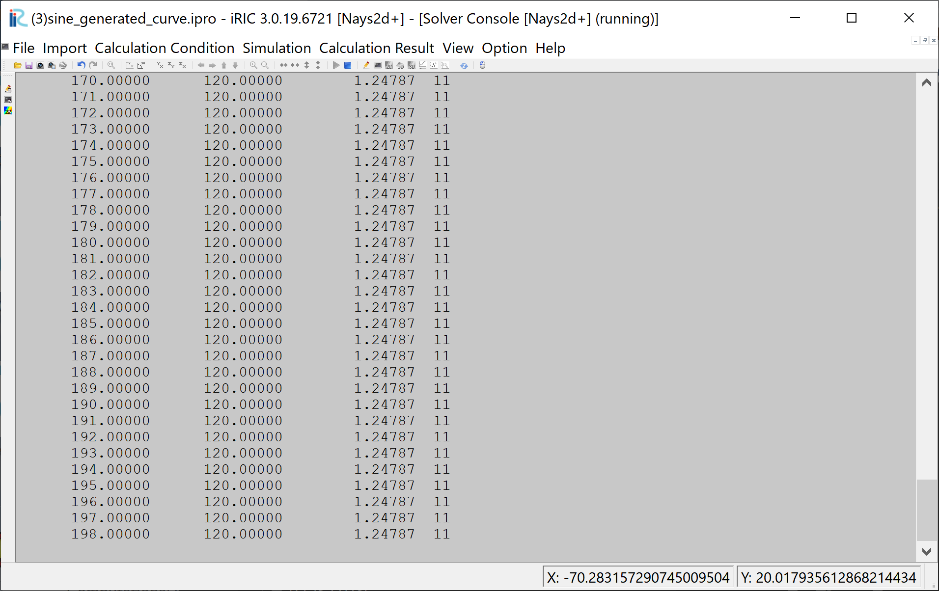
Figure 65 :Launch Computational

By selecting [Simulation] and [Run], a window as Figure 65 appears, and the simulations starts.

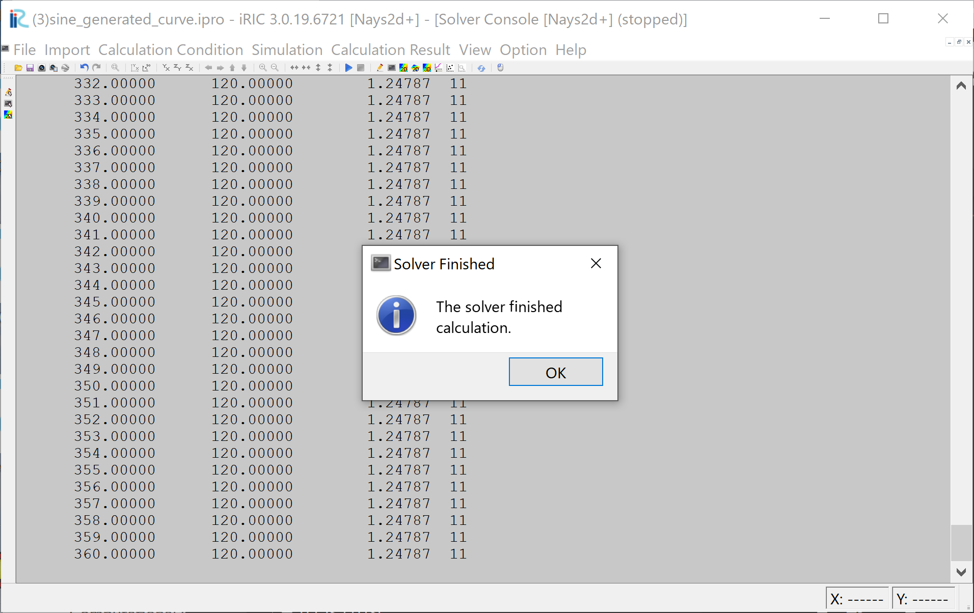
Figure 66 :Simulation Fished

When the simulation finish, Figure 66 appears. Then click [OK].

Display Computational Results

After the companion finished, form the main menu, by selecting [Calculation Results] and [Open new 2D Post-Processing Window], a new Window appears as Figure 67 .

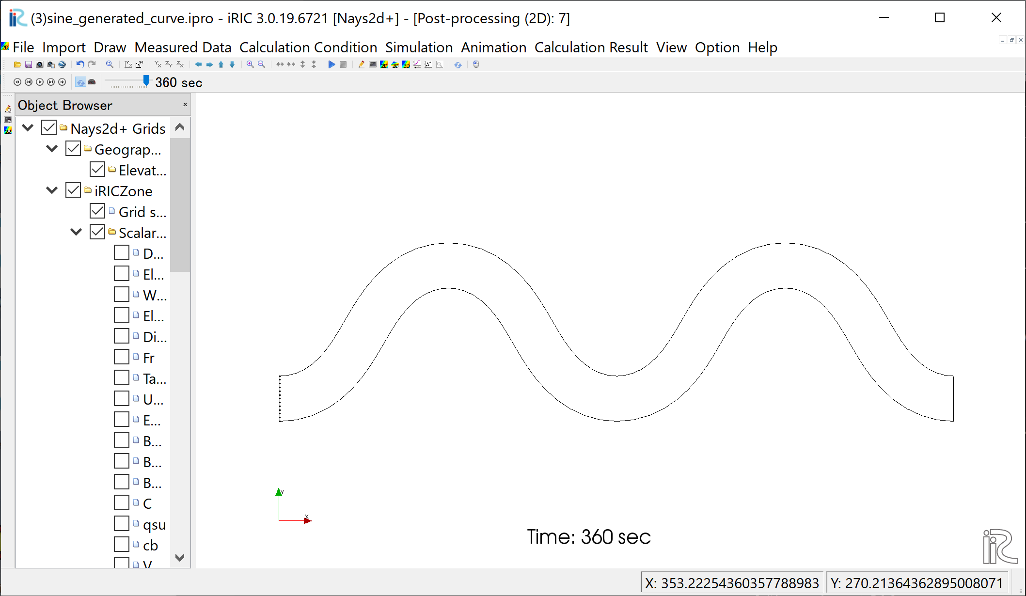
Figure 67 :2D Post-Processing Window

Depth

In the object browser, put the check marks in “Scalar (node)” and “Depth[m]”, right-click and select “Properties”. The “Scalar Setting” window Figure 68 appears.

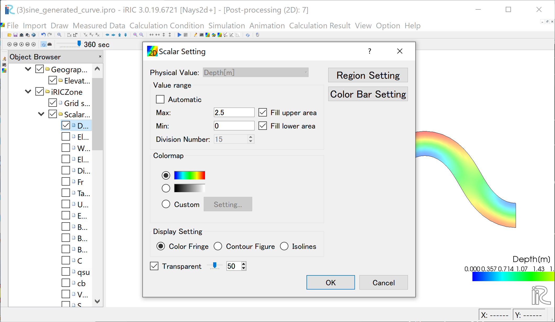
Figure 68 :Scalar Setting

Set the values as shown in Figure 68, and click [OK], then Figure 69 appears.

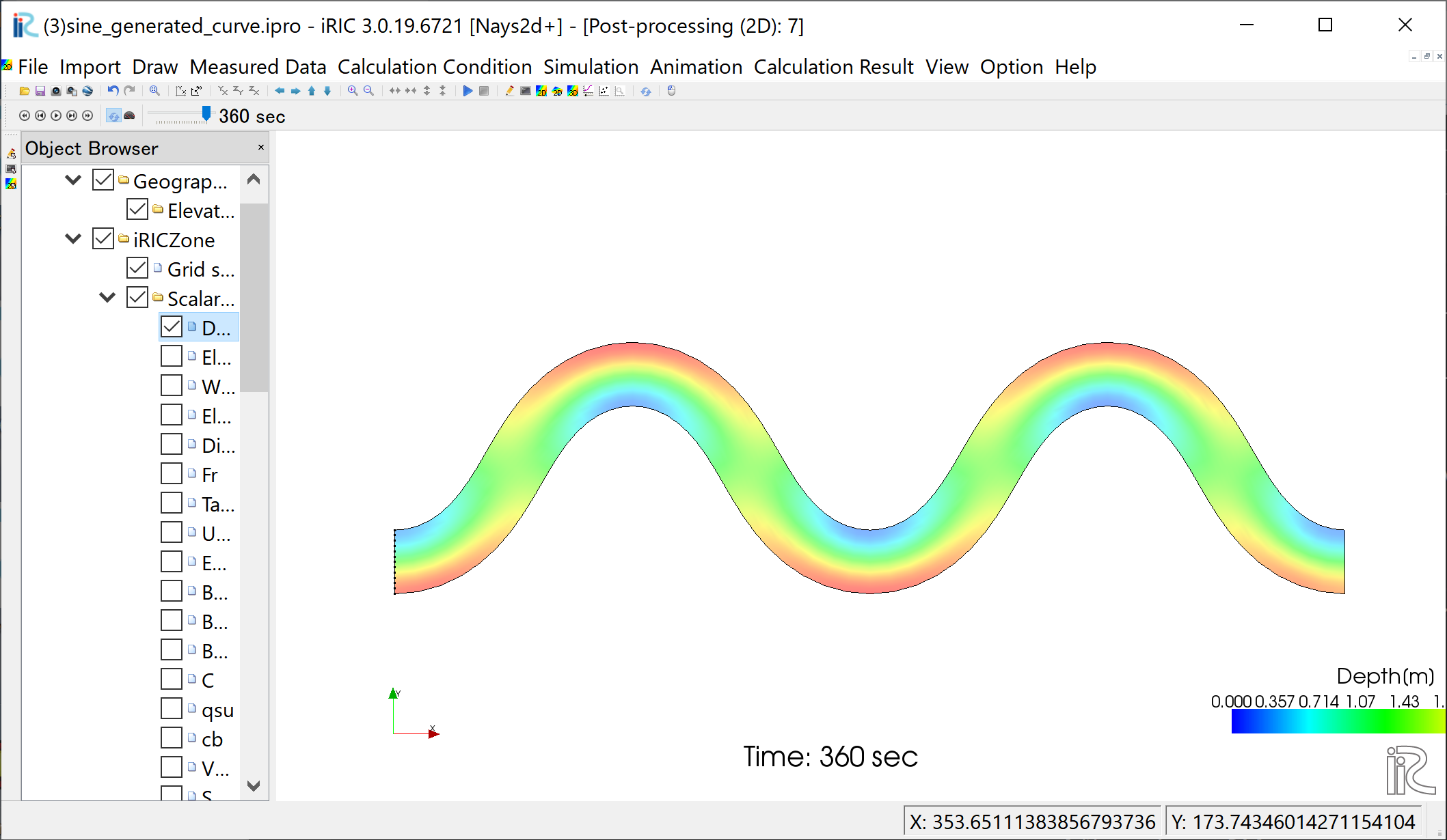
Figure 69 : Depth Plot

Velocity vectors

In the object browser, put the check marks in “Arrow” and “Velocity”, right-click and select “Properties”. The “Arrow Setting” window Figure 70 appears. Set the values as Figure 70, and click [OK].

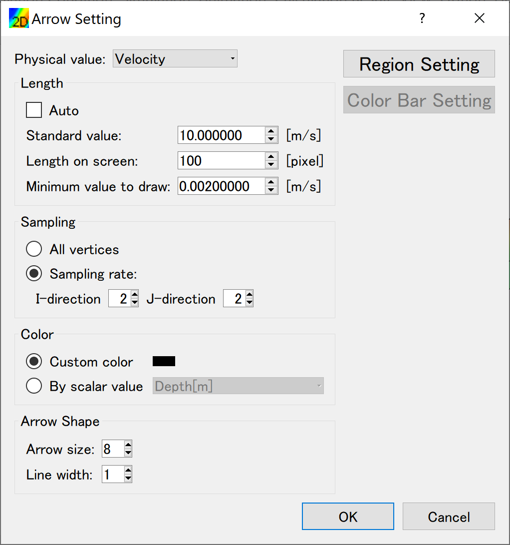
Figure 70 :Arrow Setting

Figure 71 shows the depth-averaged velocity vectors.

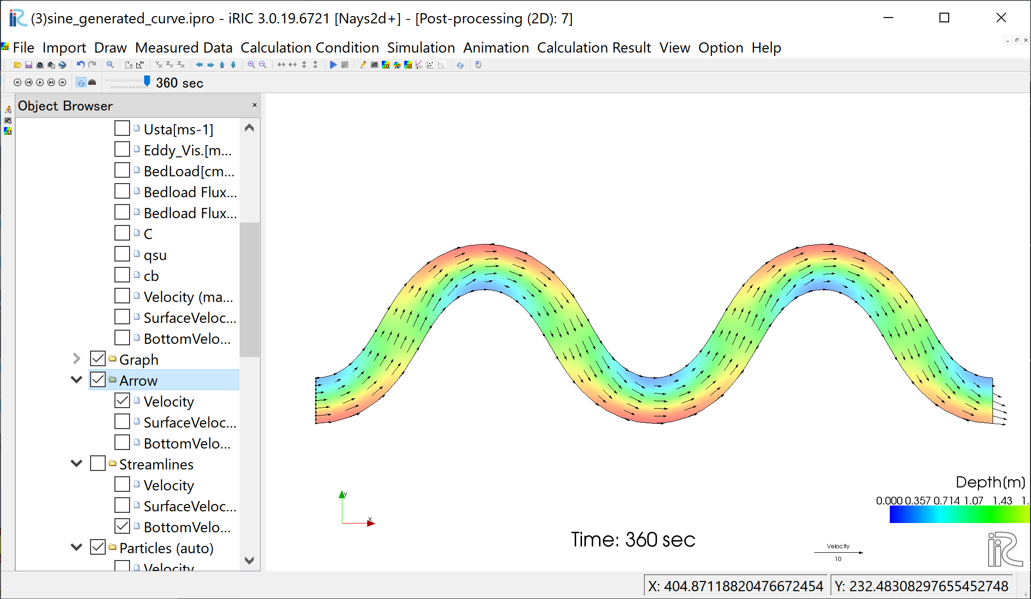
Figure 71 :Depth Averaged Velocity Vectors

In Figure 71, you can select “Surface Velocity” and “Bottom Velocity” by checking each box in “Arrow” group.

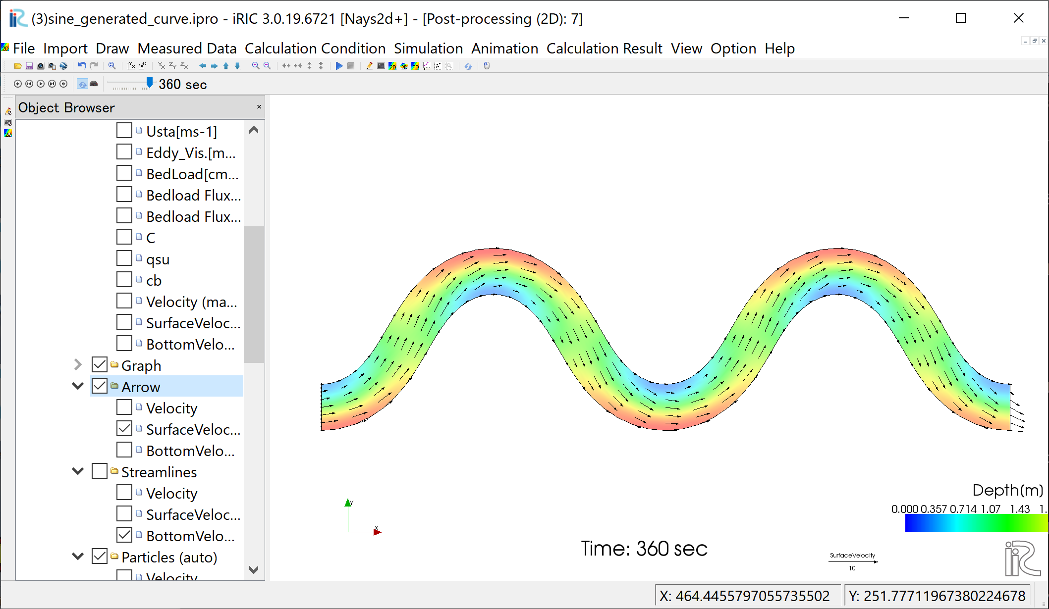
Figure 72 : Surface Velocity Vectors

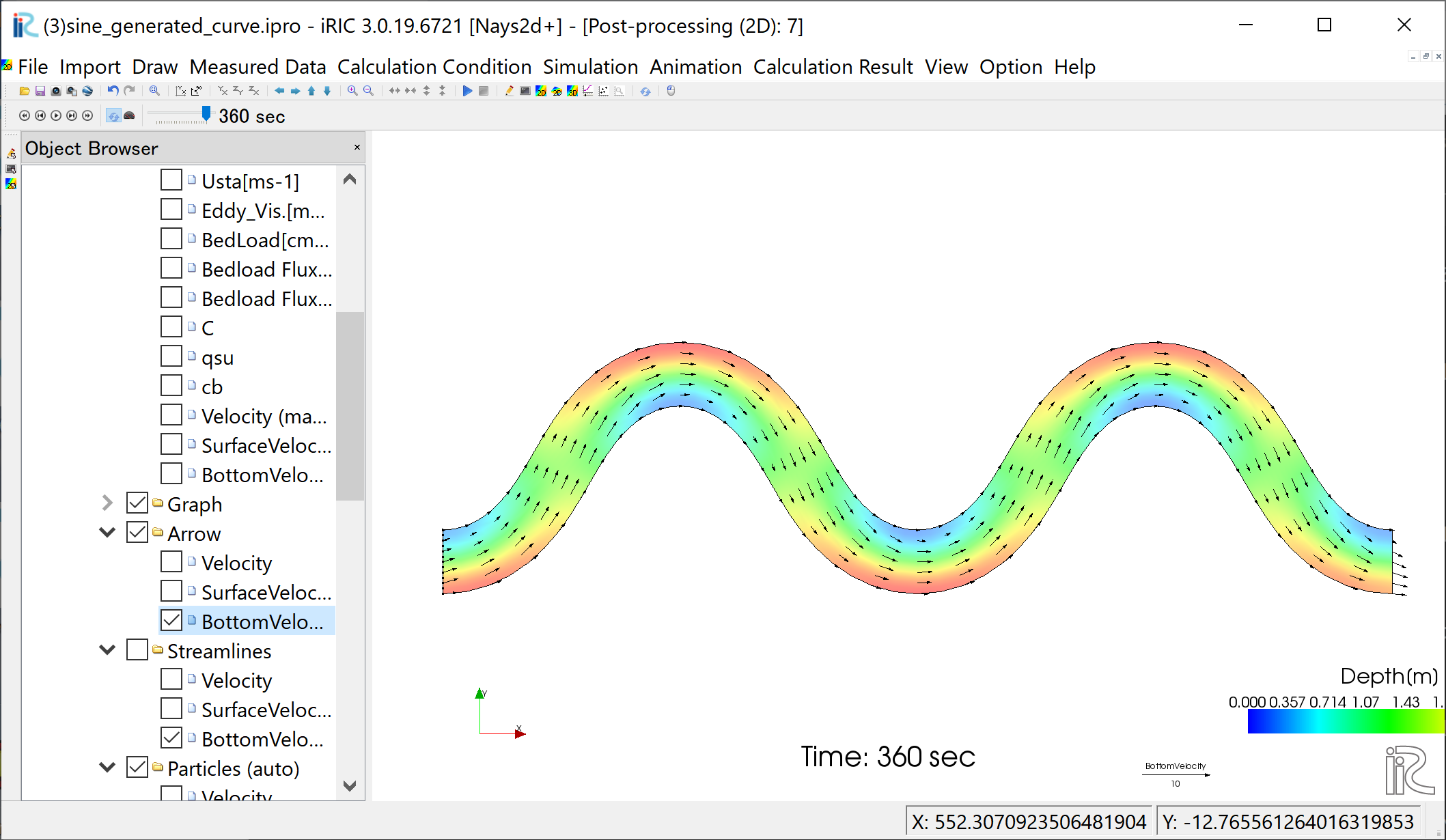
Figure 73 : Bottom Velocity Vectors

Stream Lines

Uncheck the box by “Arrow” in the Object Browser and check a box by “Streamline”. By checking “Velocity”, the streamlines following the depth averaged flow velocity” Figure 74 will be displayed. By checking “Surface Velocity”, the streamline following the surface velocity” Figure 75 will be displayed. By checking “Bottom Velocity”, the streamline following the bottom velocity ne: numref:03_kekka_11 will be displayed.

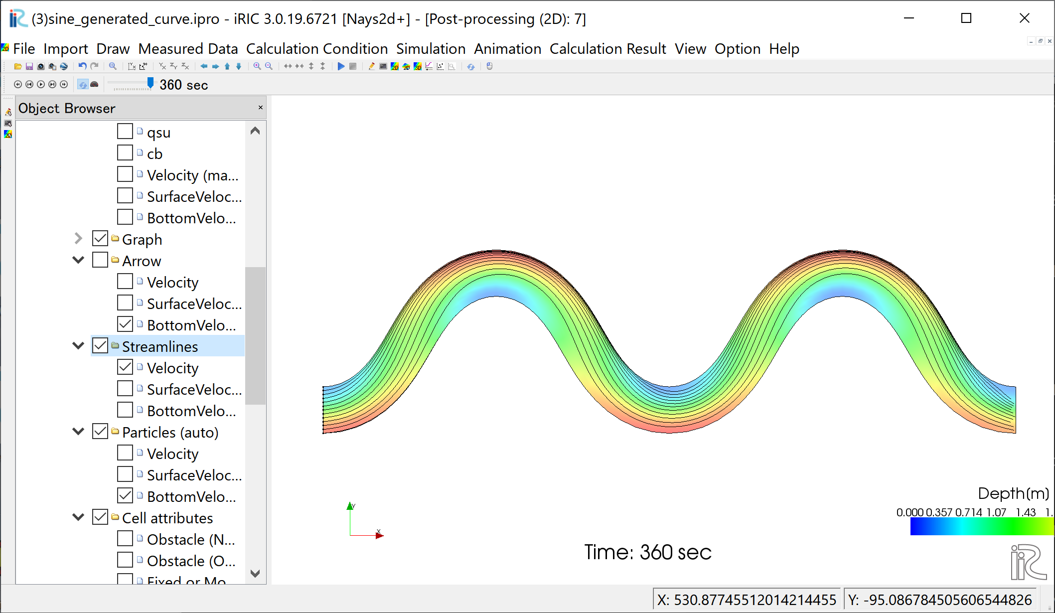
Figure 74 :Streamlines by depth averaged velocity

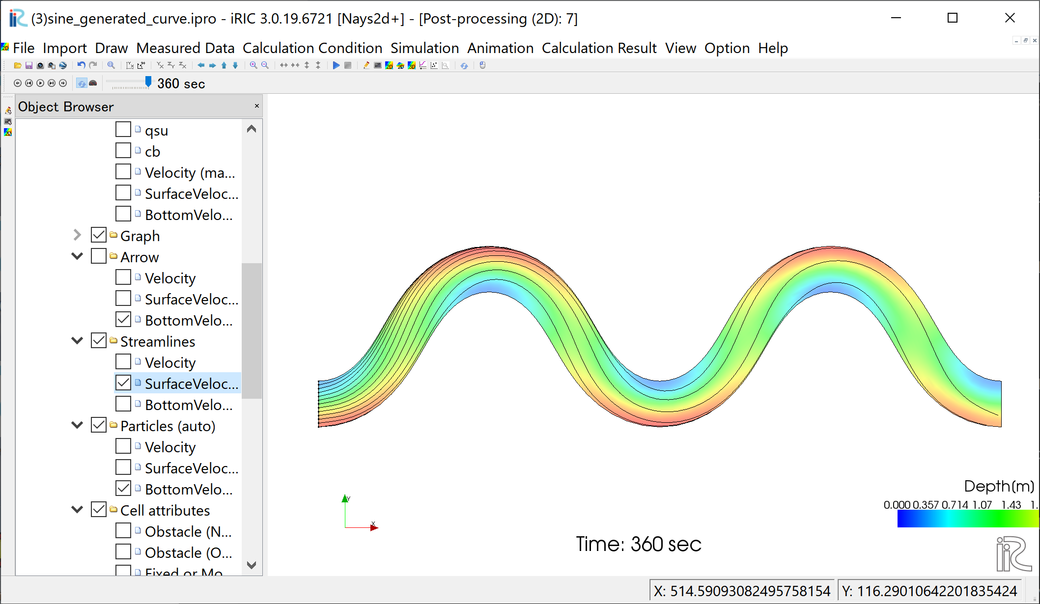
Figure 75 :Streamlines by surface velocity

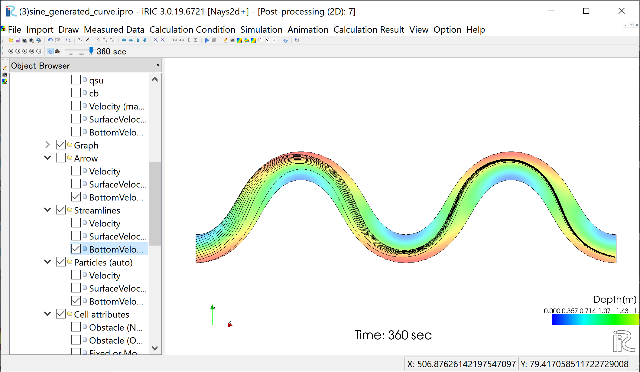
Figure 76 :Streamlines by bottom velocities

The effect of the secondary flow is clearly shown.

Particle Animation

In the object browser, uncheck the box of [Streamlines], and check the boxes of [Particles] and [Velocity], and set the time bar back to zero, as shown in Figure 77 Click small black play button, and particle animation starts as Figure 78, which shows the particles following depth averaged flow.

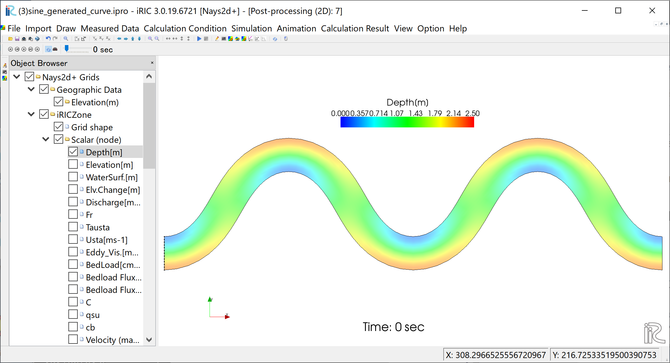
Figure 77 : Starting of Particle Animation

Figure 78 : Animation of particles following the depth averaged velocity

In the same way, the particle flowing animations can be played by checking a box at [Surface Velocity], and [Bottom Velocity], respectively.

Figure 79 : Animation of particles following the surface velocity

Figure 80 : Animation of particles following the bottom velocity