2. Basics of partial differential equations

2.1. Finite differential schemes for advection equations

One of the most basic partial differential equations that express the temporal and spatial fluid problems addressed by hydraulic engineers is the following advection equation.

(2.1)\[\cfrac{\partial f}{\partial t}+c\cfrac{\partial f}{\partial x}=0\]

Where, \(f\) is the fluid advection amount, \(x\) is the coordinate axis in the flow direction, \(t\) is the time, and \(c\) is the advection velocity. This equation expresses the state in which the variable \(f\) is transported in the direction of \(x\) at the velocity of \(c\) while maintaining its value. The theoretical solution to Equation (2.1) can be relatively easily obtained as shown in the Appendix (refer to Theoretical solutions to advection equations).

For example, the first two terms on the left side of (7.2) are included in this type of formula. You can see this type of formula on many different occasions. Now, as shown in Figure 2.1, we divide the \(x\) axis by \(\Delta x\) into 1, 2, 3, \(\cdots\), \(i-1, i, i+1\), \(\cdots\), \(N-1, N\).

We also divide the \(t\) axes by \(\Delta t\) into 1, 2, 3, \(\cdots\), \(j-1, j, j+1, \cdots, J-1, J\).

Then, if we assume that \(f\) at \((x, t)\) is \(f(i,j)\), and \(f\) at \((x+\Delta x, t+\Delta t)\) is \(f(i+1,j+1)\), then we have…

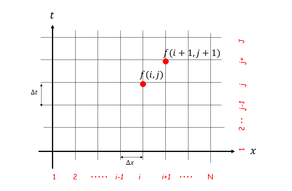
Figure 2.1 : Placement of discrete variable in the space (\(x\), \(t\))

The first term in Equation (2.1) expresses a temporal sequence. Then, generally it is expressed as follows.

(2.2)\[\cfrac{\partial f}{\partial t} = \cfrac{f(i,j+1)-f(i,j)}{\Delta t}\]

The second term expresses the spatial differentiation. There are the following three schemes that can be considered simple.

(2.3)\[c\cfrac{\partial f}{\partial x} = c\cfrac{f(i+1,j)-f(i,j)}{\Delta x} \; \; \; \; \; \mbox{[forward difference scheme]}\]

(2.4)\[c\cfrac{\partial f}{\partial x} = c\cfrac{f(i,j)-f(i-1,j)}{\Delta x} \; \; \; \; \; \mbox{[backward difference scheme]}\]

(2.5)\[c\cfrac{\partial f}{\partial x} = c\cfrac{f(i+1,j)-f(i-1,j)}{2\Delta x} \; \; \; \mbox{[central difference scheme]}\]

Considering the directions of these three difference schemes, Equation (2.3) is called [forward difference scheme], Equation (2.4) is called [backward difference scheme], and Equation (2.5) is called [central difference scheme].

[Central difference scheme] may seem the most intuitively accurate. But is it? Let us check which scheme gives the most accurate solutions in the following section.

2.2. Differences in solutions by difference method

2.2.1. Backward difference scheme (The Python code and calculation results)

Of the three difference schemes listed above, let us try the backward difference scheme first. Substituting Equation (2.2) and Equation (2.4) into Equation (2.1) gives us…

(2.6)\[f(i,j+1)=f(i,j)-c\cfrac{f(i,j)-f(i-1,j)}{\Delta x}\Delta t\]

To show the temporal and the spatial calculation range in an easily understandable way, we adopted the two-dimensional space of \((i,j)\), as shown by Figure 2.1. However, in the actual calculation, once you calculate \(j \Rightarrow j+1\), you no longer need variables for \(j\). By coding this process as shown below, \(f\) becomes a 1D problem.

for i in range(1,N+1):
    fn[i]=f[i]-c*(f[i]-f[i-1])*dt/dx
f=fn

Calculate \(f\) (here we assume it to be fn[i]) for a new “time”, then replace it with the \(f\) of the old “time” and calculate the \(f\) for the next time step.

Then, repeat this process.

The Python code for calculating the advection equation with a backward difference scheme is…

https://github.com/YasuShimizu/Python-Code/blob/main/backward.py

The calculation that results from this code is shown below. The initial distribution of \(f\) is assumed to be a triangular distribution and is shown in Figure 2.3. Where, \(x_p\) =10, \(x_b\) =10, \(f_p\) =0.5, and \(c\) =0.5.

Figure 2.2 : Calculation results for the backward difference scheme (\(c>0\))

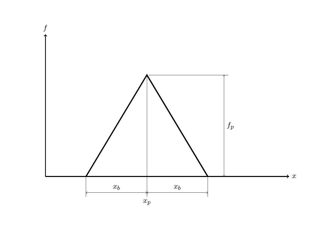
Figure 2.3 : Initial distribution of \(f\)

You may have noticed from Figure 2.2 that the solutions to this equation show the peak of the triangular distribution to gradually become smaller and the distribution shape to change, even though, as shown by Figure 1 of Appendix, the triangular distribution should be maintained while it moves at a velocity of \(c\).

The reasons will be explained later. Now, we make calculations using the forward difference scheme and the central difference scheme.

2.2.2. The forward difference scheme (The Python code and calculation results)

Substituting Equation (2.2) and Equation (2.3) into Equation (2.1) gives us the time-updated formula of \(f\) using forward difference scheme as follows.

(2.7)\[f(i,j+1)=f(i,j)-c\cfrac{f(i+1,j)-f(i,j)}{\Delta x}\Delta t\]

The Python code for this section is…

for i in range(1,N+1):
    fn[i]=f[i]-c*(f[i+1]-f[i])*dt/dx
f=fn

The source code is…

https://github.com/YasuShimizu/Python-Code/blob/main/forward.py

The calculation result for this code diverges (‘ω’).

Figure 2.4 : Calculation results for the forward difference scheme (\(c>0\))

2.2.3. Central difference scheme (The Python code and calculation results)

Substituting Equation (2.2) and Equation (2.5) into Equation (2.1) gives us the time-updated formula of using forward difference scheme as follows.

(2.8)\[f(i,j+1)=f(i,j)-c\cfrac{f(i+1,j)-f(i-1,j)}{2 \Delta x}\Delta t\]

The Python code is…

https://github.com/YasuShimizu/Python-Code/blob/main/central.py

The calculation result is…

Figure 2.5 : Calculation results for the central difference scheme (\(c>0\))

In this case, the triangle seems to move at a constant velocity while keeping the value of the peak. However, the noise that’s generated backwards increases until the peak of noise exceeds the peak of the triangle, which is an unrealistic value.

2.2.4. Summary

Our comparison of the three difference schemes found the following.

• None of them reproduce the theoretical solutions.

• Although the backward difference scheme gives stable solutions, the solutions are inaccurate due to reductions in the peak values and for other reasons.

• The central difference scheme maintains the initial distribution shape. However, it generates a lot of noise.

• The solutions of the forward difference scheme diverge soon after the calculation starts.

2.3. Advection direction and difference schemes

The above discussions were for cases when the advection velocity, \(c\), is positive. Next, let us examine the cases of \(c<0\).

2.3.1. The Python code and calculation results

Here, the calculation results for \(c<0\) and the The Python code that correspond each case.

Figure 2.6 : Calculation results for the backward difference scheme (\(c<0\))

https://github.com/YasuShimizu/Python-Code/blob/main/backward-.py

Figure 2.7 : Calculation results for the forward difference scheme (\(c<0\))

https://github.com/YasuShimizu/Python-Code/blob/main/forward-.py

Figure 2.8 : Calculation results for the central difference scheme (\(c<0\))

https://github.com/YasuShimizu/Python-Code/blob/main/central-.py

Consequently, the features of the three difference schemes for \(c>0\) and \(c<0\) are summarized in the following table.

Table 2.1 Summary of the three difference schemes

Difference scheme	Backward (\(i\) and \(i-1\))	Forward (\(i\) and \(i+1\))	Central (\(i-1\) and \(i+1\))
When \(c>0\)	Stable but inaccurate	Divergence	Unstable but fairly accurate
When \(c<0\)	Divergence	Stable but inaccurate	Unstable but fairly accurate

Therefore, stable calculation can be expected only for the backward difference scheme when \(c>0\) and for the forward difference scheme when \(c<0\). These two schemes–the difference schemes in which the position data of i and i-1 are used when \(c>0\) and in which i and i+1 are used when \(c<0\)– are called the upwind difference scheme, analogous to the naming convention for wind directions \(c\).

The concept of upwind difference scheme is very important for numerical calculation. It means performing difference calculation in the direction of the information that is forwarded. However, the simple upwind difference schemes shown here have the shortcoming of providing stable but not highly accurate calculations.

The reasons for this shortcoming will be discussed later. Next, we’ll talk about numerical solutions to diffusion equations, which in addition to advection equations, are important equations.

2.4. Finite differential scheme for a diffusion equation

Another important basic formula for fluid calculation is the diffusion equation shown below.

(2.9)\[\displaystyle{{{\partial f}\over{\partial t}}=D{{\partial^2 f}\over{\partial x^2}}}\]

Where, \(D\) is the diffusion coefficient. Now, let us discuss the meaning of Equation (2.9).

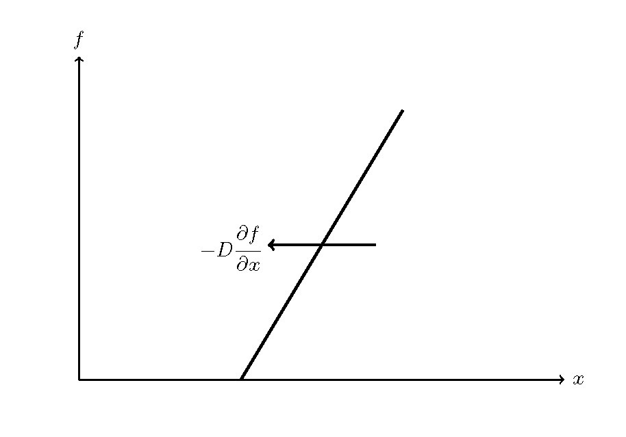
Figure 2.9 : Diffusion equation (1)

Let us assume, as shown in Figure 2.9, that \(f\) is the density, that the density gradient \(\cfrac{\partial f}{\partial x}\) occurs, that density transport is generated in the direction from high density to low density, that density transport is proportional to the density gradient, and that the proportional coefficient is \(D\), then the flux is expressed as \(-D\cfrac{\partial f}{\partial x}\).

When the gradient is positive, flux transport is generated in the direction opposite to the \(x\) axis. Therefore, please note that a positive transport volume is expressed in a negative value, thus put a minus sign, “-”.

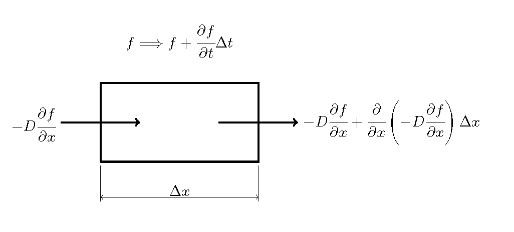
Figure 2.10 : Diffusion equation (2)

As shown in Figure 2.10, we assume that the differences in the flux are caused by the density gradient between two points that are separated by the distance of \(\Delta x\). Such differences in flux generate density changes, \(f \Longrightarrow f+\cfrac{\partial f}{\partial t}\Delta t\), during time, \(\Delta t\). Then, we have…

(2.10)\[\left( \cfrac{\partial f}{\partial t}\Delta t \right) \Delta x =\left\{ \cfrac{\partial}{\partial x}\left(-D\cfrac{\partial f}{\partial x} \right) \Delta x \right\} \Delta t\]

We divide both sides of Equation (2.10) by \(\Delta x\) and \(\Delta t\), and we assume that \(D\) is a constant, then we have Equation (2.9).

The second derivative on the right side of (2.9) is obtained by first differentiating at both upper and lower sides of the calculation point and then differentiating them again. Therefore…

(2.11)\[\begin{split}D \cfrac{\partial^2 f}{\partial x^2}= \cfrac{D}{\Delta x} \left(\cfrac{f(i+1,j)-f(i,j)}{\Delta x} - \cfrac{f(i,j)-f(i-1,j)}{\Delta x}\right) \\ =\cfrac{D}{\Delta x^2}\Bigl\{f(i+1,j)-2f(i,j)+f(i-1,j)\Bigr\}\end{split}\]

If we assume that the differentiation of the left side in terms of time is simply the time difference, then the difference of (2.9) is expressed by the following equations.

(2.12)\[\cfrac{f(i,j+1)-f(i,j)}{\Delta t}= \cfrac{D}{\Delta x^2}\Bigl\{f(i+1,j)-2f(i,j)+f(i-1,j)\Bigr\}\]

or

(2.13)\[f(i,j+1)=f(i,j)+ D \cfrac{\Delta t}{\Delta x^2} \Bigl\{f(i+1,j)-2f(i,j)+f(i-1,j)\Bigr\}\Delta t\]

As we did for the advection equation in the previous section, we obtain the following, where f and fn are calculated by the successive interchanging of f and fn.

for i in range(1,N+1):
    fn[i]=f[i]+D*(f[i+1]-2*f[i]+f[i-1])*dt/dx**2
f=fn

2.4.1. The Python code and calculation results

The entire source code is here. In addition, the calculation results when \(D=0.8\) are shown by Figure 2.11.

https://github.com/YasuShimizu/Python-Code/blob/main/diffusion.py

Figure 2.11 : Calculation results for the diffusion equation

Because Figure 2.11 expresses the situations where the peak becomes smaller and the distribution become wider, the situation is actually the diffusion phenomena. Thus, it is relevant.

You may have noticed that Figure 2.2 and Figure 2.7, which are equivalent to the upwind difference scheme, diffuse similarly.

The solutions to the advection equation are not supposed to diffuse in this way but are supposed to move while maintaining the initial distribution shape (Figure 1).

For some reason, diffusion occurs at the same time as advection. In this way, the solutions to the advection equation are known to diffuse by “numerical calculation”, despite such diffusion not occurring in reality.

Such diffusion is called “numerical diffusion” to distinguish it from the diffusion in real flow situation. Now, let us consider why such “numerical diffusion” occurs.

2.5. Numerical diffusion caused by upwind differential shame

The upwind difference scheme needs to change direction according to the direction of advection, or to the sign (+/-) of the value of \(c\). In coding, it’s sufficient to use “if” statements to make decisions each time, but explanations of the features are easier to understand when “if” statements are not used.

Here, let me introduce a method that expresses the upwind difference scheme without “if” statements. First, let us consider the following equations.

(2.14)\[ \begin{align}\begin{aligned}\begin{split}c + |c| = \Bigl\{ \begin{matrix} 2c & ;(c>0) \\ 0 & ;(c<0) \\ \end{matrix} \\\end{split}\\\begin{split}c - |c| = \Bigl\{ \begin{matrix} 0 & ;(c>0) \\ 2c & ;(c<0) \\ \end{matrix}\end{split}\end{aligned}\end{align} \]

Therefore,

(2.15)\[ \begin{align}\begin{aligned}\begin{split}\cfrac{1}{2}(c + |c|) = \Bigl\{ \begin{matrix} c & ;(c>0) \\ 0 & ;(c<0) \\ \end{matrix} \\\end{split}\\\begin{split}\cfrac{1}{2}(c - |c|) = \Bigl\{ \begin{matrix} 0 & ;(c>0) \\ c & ;(c<0) \\ \end{matrix}\end{split}\end{aligned}\end{align} \]

Considering the features of Equation (2.15), we assume the following equations.

(2.16)\[F=\cfrac{1}{2}(c + |c|)\cfrac{f(i)-f(i-1)}{\Delta x}+ \cfrac{1}{2}(c - |c|)\cfrac{f(i+1)-f(i)}{\Delta x}\]

From Equation (2.15) and Equation (2.16),

(2.17)\[\begin{split}F=\Biggl\{ \begin{matrix} c \cfrac{f(i)-f(i-1)}{\Delta x} & ;(c>0) \\ c \cfrac{f(i+1)-f(i)}{\Delta x} & ;(c<0) \\ \end{matrix}\end{split}\]

Therefore,

(2.18)\[\cfrac{\partial f}{\partial t}+F=0\]

or

(2.19)\[\cfrac{f_n(i)-f(i)}{\partial t} + \cfrac{1}{2}(c + |c|)\cfrac{f(i)-f(i-1)}{\Delta x}+ \cfrac{1}{2}(c - |c|)\cfrac{f(i+1)-f(i)}{\Delta x} =0\]

is an equation that expresses the upwind difference scheme without using “if” statements. Where, \(f_n(i)\) and \(f(i)\) respectively express \(f(i,j+1)=f(x,t+\Delta y)\) and \(f(i,j)=f(x,t)\).

From Equation (2.19), the upwind difference scheme can be expressed by

(2.20)\[f_n(i)=f(i)- \underbrace{ \cfrac{c \Delta t}{2 \Delta x}\left\{ f(i+1)-f(i-1) \right\} }_{a} + \underbrace{ \cfrac{|c|\Delta t}{2 \Delta x} \left \{ f(i+1)-2f(i)+f(i-1) \right\}}_{b}\]

Now, let us rewrite the central difference scheme in the advection equation of Equation (2.8) and the difference scheme of the diffusivity equation, Equation (2.13), with the same form, the central difference scheme of advection equation is

(2.21)\[f_n(i)=f(i)-\underbrace{ \cfrac{c \Delta t}{2 \Delta x} \left\{{f(i+1)-f(i-1)} \right\}}_{a'}\]

The diffusivity equation is

(2.22)\[f_n(i)=f(i)+ D \cfrac{\Delta t}{\Delta x^2} \Bigl\{f(i+1)-2f(i)+f(i-1)\Bigr\}\]

Here, assuming that \(D=\cfrac{|c|\Delta x}{2}\), we obtain

(2.23)\[f_n(i)=f(i)+\underbrace{ \cfrac{|c|\Delta t}{2\Delta x} \Bigl\{f(i+1)-2f(i)+f(i-1)\Bigr\}}_{b'}\]

You can see that a in the Equation (2.20) is corresponding to a’ in the Equation (2.21), as well as b in Equation (2.20) is corresponding to the b’ of Equation (2.23).

The (a+b) part of the upwind difference scheme expressed by Equation (2.20) can be divided into a central difference scheme (a’) and a diffusion equation (b’ ). Consequently, it’s in the form of their addition. The diffusion of the b part is initially an advection equation. Therefore, despite the diffusion of b not being included in reality, it is an element automatically included when we perform the upwind difference scheme.

This is called “numerical diffusion” because it is included when numerical calculations are performed, in contrast to the original physical phenomena of “diffusion”. This is what “numerical diffusion” really is.

Figure 2.2 and Figure 2.7 correspond to the upwind difference scheme. They are characterized by a central difference scheme that moves at a constant velocity while maintaining its shape and by diffusion whose peak decreases while its shape widens.

This upwind difference scheme gives solutions that are stable but inaccurate. What we want are calculation results that are close to the theoretical values, as shown by Figure 1. So, in the next chapter, I will explain difference schemes that keep “numerical diffusion” as low as possible.