12. Calculation of 2D flow and bed deformation in meandering channels (basic edition)
12.1. Secondary flow and the direction of bottom shear stress
12.1.1. What is a secondary flow?
When calculating bed deformation using 2D planar calculations, the velocity vector near the bed bottom that takes secondary flows into account is important, in addition to the velocity vector that is obtained from the depth-averaged flow calculation. This is because the direction of sediment transport is important in bed deformation calculations and because the direction of sediment transport is determined by the direction of near-bottom current velocities. Usually, curved flow in a plane generates centrifugal forces that in turn generate secondary flows, called spiral secondary flows, whose axes are oriented in the direction of the streamline. Flow in the original flow direction, downstreamward, is called the main flow, in contrast to secondary flows.
Note
Previous chapters treated the flow field as a depth-averaged flow field. For example, \(u_s\) represents the depth-averaged flow velocity in the \(s\) axis direction. However, hereinafter, in descriptions of secondary flows, the flow velocity also has a distribution in the depth direction. Therefore, \(u_s\) is not used as a depth-averaged value, but as a value with a distribution in the depth direction. The depth-averaged velocity is from values distributed in the depth direction. Therefore, it is expressed as \(<u_s>\) in \(<\;>\). Because the wording is confusing, please read it carefully.
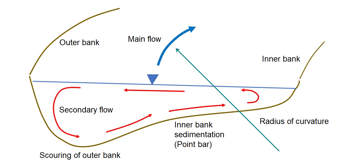
Figure 12.1 : Secondary flows
For example, when a channel is curved, as shown in Figure 12.1, the main flow bends along the channel, resulting in centrifugal forces that are described by the following equation.
Where, \(F_s\) is the centrifugal force, \(u_s\) is the velocity in the main flow direction, and \(r\) is the radius of curvature at a bend of the main flow. The vertical velocity of the main flow is high near the water surface where there is no resistance but is low near the bed, where it is influenced by bottom traction, similar to the well-known logarithmic law and the parabolic distribution. Therefore, as in Equation (12.1), the centrifugal force that is proportional to the square of the flow velocity is overwhelmingly great near the water surface, so the secondary flows on the water surface are directed towards the outer bank. Compensating for this motion (to satisfy the equation of continuity), flows towards the inner bank occur at the bottom, resulting in secondary flows that circulate across the entire cross-section. The scouring on the outer banks of a movable bed channel and the deposition of sedimentation and the formation of sandbars on the inner banks are mainly due to secondary flows.
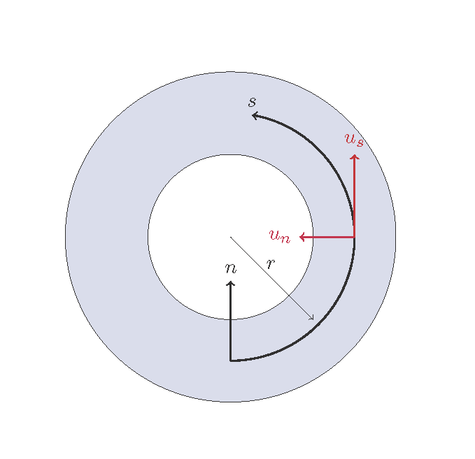
Figure 12.2 : Uniform bend flow in a concentric channel
When examining the characteristics of a secondary flow, the simplest state of the flow is a uniform bend flow, as shown in Figure 12.2, which makes the analytical process easy. This situation assumes a channel where the left and right banks are in concentric circles with a constant gradient (a hypothetical situation where the concentric circles spiral endlessly because of the gradient). In this hypothetical channel, we assume uniform flow with a constant discharge. It is clear that the streamlines for all depth-averaged flows also can be drawn as concentric circles. Therefore, it is obvious that \(<u_s>\) is the uniform flow velocity and that \(<u_n>=0\).
Many researchers have proposed equations to express the velocity distribution of secondary flows in the main flow such as uniform bend flow (uniform flow with a constant radius of curvature). Here, we introduce an equation proposed by Engelund [Ref:38] for secondary flow distribution, shown below. For the derivation of the equation, please refer to Appendix V (Appendix V (The main flow and the secondary flow velocity distribution by Engelund [Ref:38] )).
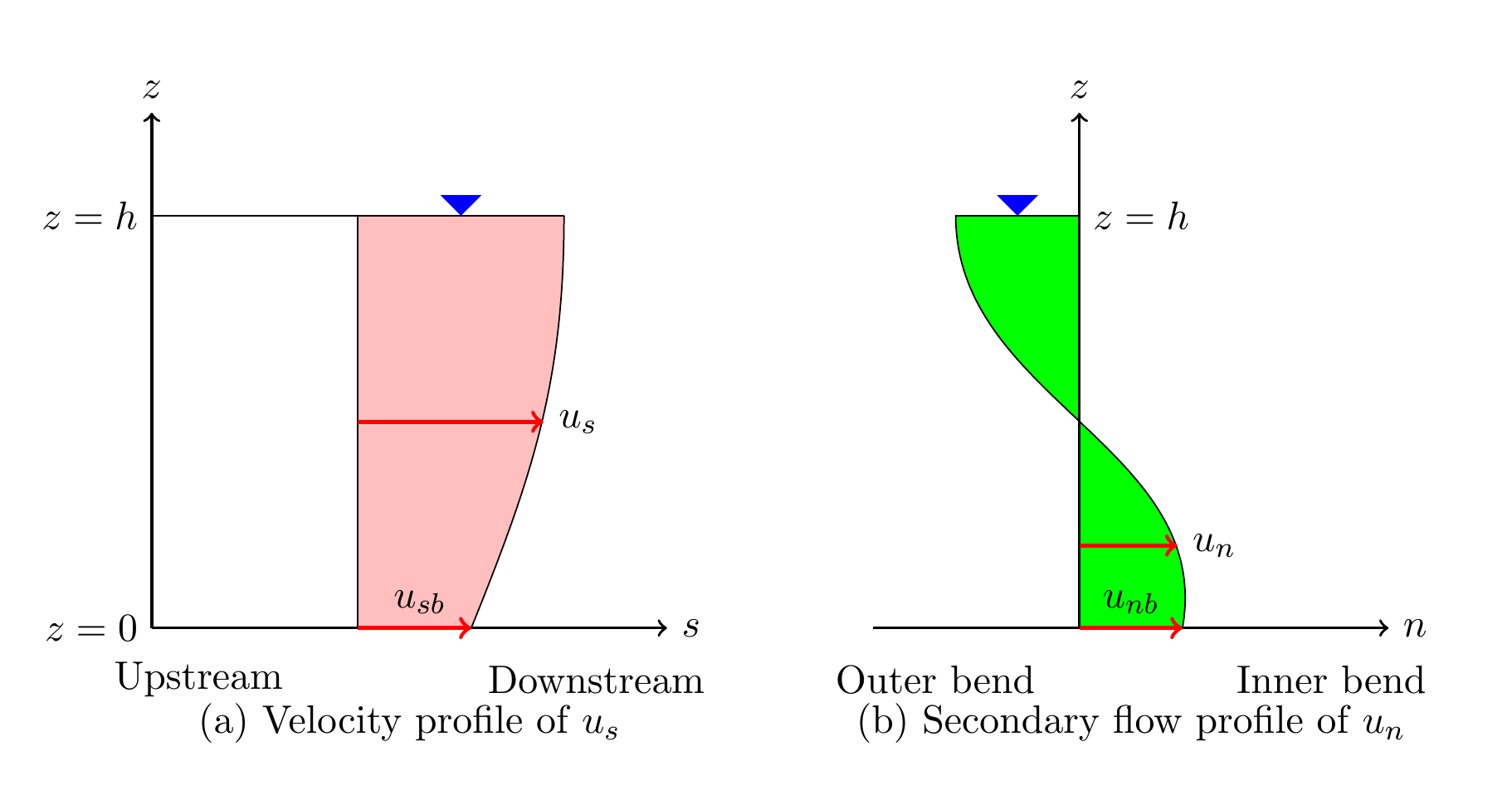
Figure 12.3 : Velocity distributions of the main flow and the secondary flows
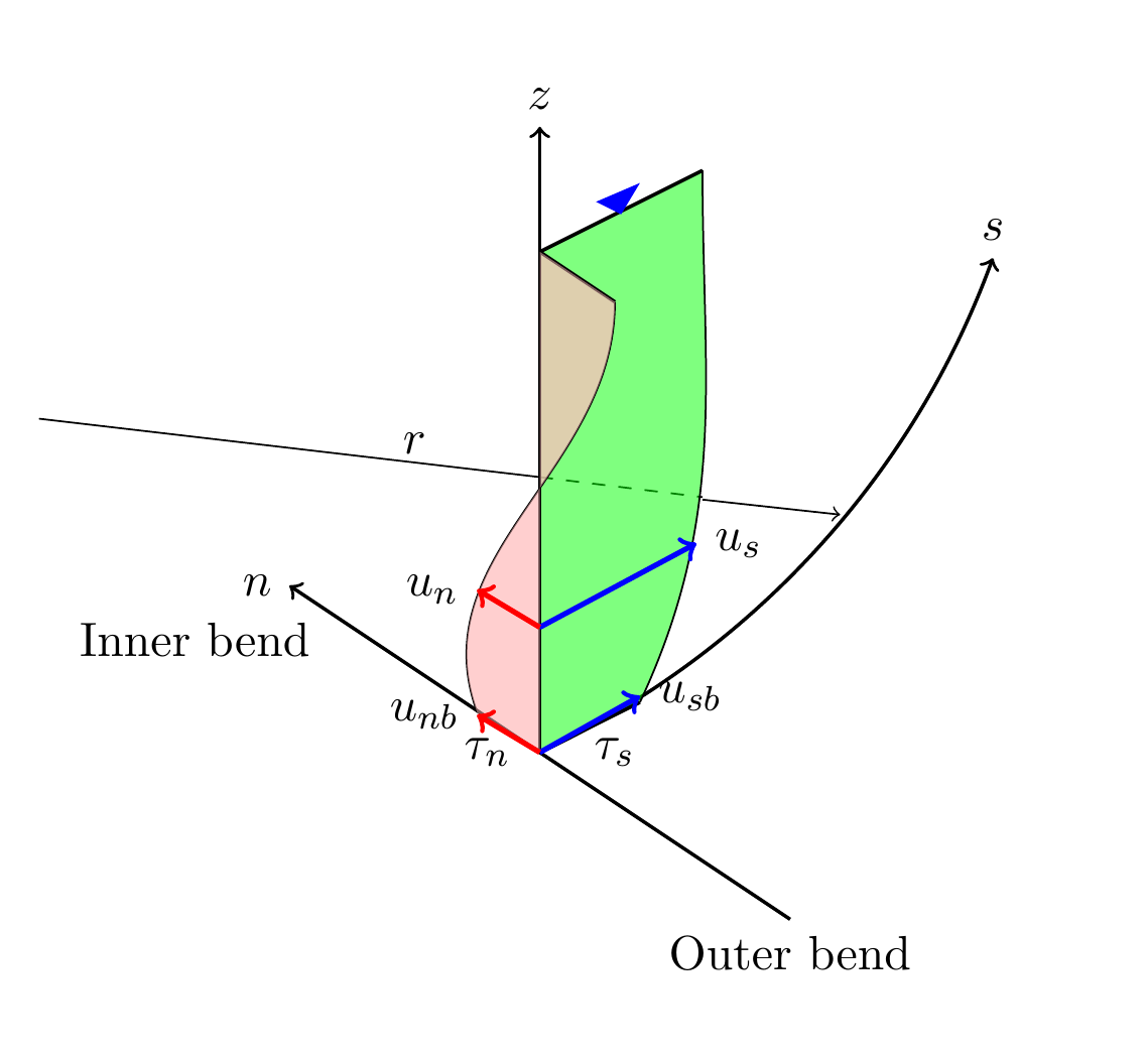
Figure 12.4 : Velocity distributions of the main flow and the secondary flows (3D)
12.1.2. Distribution of vertical velocities for the main flow (parabolic distribution)
Where, \(u_s\) is the flow velocity in the flow direction, \(<u_s>\) is the average water depth of \(u_s\), and \(zeta\) is the non-dimensional distance from the bed as expressed by the following equation.
Where, \(z\) is the distance from the bed, \(z_b\) is the bed elevation and \(h\) is the water depth. \(\chi\) and \(\chi_1\) are constants. Refer to this link for a method of calculating them.
12.1.3. Velocity distribution of secondary flows (6D distribution function)
Where, \(u_n\) is the flow velocity in the cross-sectional direction and \(A_n\) is given by the following equation.
Where,
Regarding the variables that appear in (12.4), (12.5), and (12.6), please refer to this link.
12.1.4. Secondary flow intensity
Assuming that \(\zeta=0\) (bottom) in Equation (12.2) and Equation (12.4), and that these equations give bottom flow velocities in the \(s\) direction and in the \(n\) direction, respectively, then the ratio between them is expressed as follows.
Where, \(u_{sb}\) and \(u_{nb}\) are the values of \(u_s\) and \(u_n\) at the bottom, respectively (refer to Figure 12.3), and \(r\) and \(h\) are the radius of curvature and the water depth of the channel. \(N_\ast\) is a parameter that assumes a uniform bend flow as shown in (194). As shown in Secondary flow intensity, when we apply a general value, we have \(N_\ast \approx 7\).
Note that in reality Equation (12.7) becomes the following.
This is because the driving force of the secondary flows \(F_s\), given by Equation (12.1), is proportional to the square of the main flow, \(u_s\), and is therefore independent of the sign of \(u_s\).
Assuming that the direction of the bottom velocity also coincides with the direction of bedload transport, the following equation is valid.
Where, \(q_{bs}, q_{bn}\) are tractional load in the \(s, n\) directions.
According to Equation (12.9), in a uniformly bending channel, the presence of bedload transport in the streamline direction results in transverse sediment transport from the outer bank to the inner bank. The magnitude of the transverse sediment transport is proportional to the water depth \(h\) and is inversely proportional to the radius of curvature \(r\) of the concentric flow. This bedload transport brings sediment from the outer bank to the inner bank in a bend channel, resulting in the development of sandbars at the inner bank.
12.2. Streamline curvature
The above description is for secondary flows with uniform bend flow. How about in an ordinary meandering channel? In uniform bend flow, such as Figure 12.2, the streamline is parallel to the channel. Then, the radius of curvature is the radius of one of these concentric circles. However, in the case of meandering channels such as Figure 11.7, the streamline is obviously not parallel to the channel. The streamline has a different alignment from the alignment of the channel, and these have a phase difference.
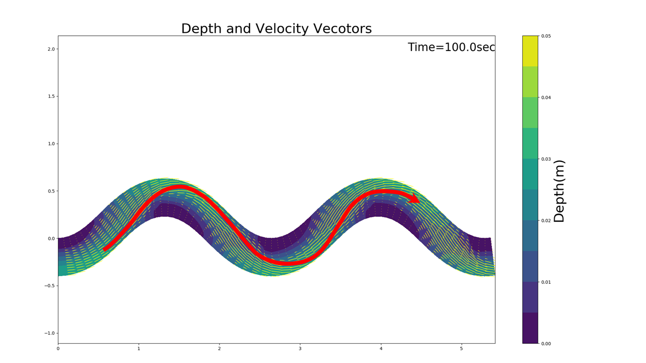
Figure 12.5 : The streamline in a meandering channel
Figure 12.5 visually represents the approximate streamline that is drawn on the vector diagram created from the calculation results. The actual streamline is estimated to be like this. Along this streamline (or more accurately, the streamline of the depth-averaged flow), no flow that crosses the streamline can be generated. Once the exact shape of this streamline is determined, by assuming this streamline to be the \(s\) axis of Figure 12.4, the secondary flows become components perpendicular to the streamline, and they can be applied to the above theoretical equation. The following explains how to calculate this ‘depth-averaged streamline’ (the red line in Figure 12.5).
12.2.1. Calculation method for streamline sinuosity
Note
The streamline here is the streamline of the depth-averaged velocity on a 2D plane. The depth-averaged velocity is used to calculate the streamline. Therefore, \(u_x, u_y, u_s, u_n\) etc. are the depth-averaged velocities.
12.2.1.1. Cartesian linear coordinates
To simplify the context, let us first assume the case of Cartesian straight coordinates (\(x-y\) coordinates).
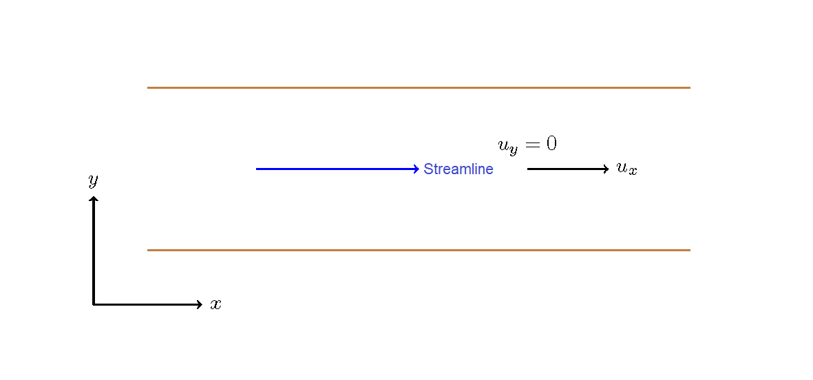
Figure 12.6 : A straight streamline in a straight channel
When the flow in a straight channel is straight, as in Figure 12.6, the streamline is as straight as the channel is, and the streamline has a curvature of zero. (The radius of curvature is infinite (\(\infty\).))
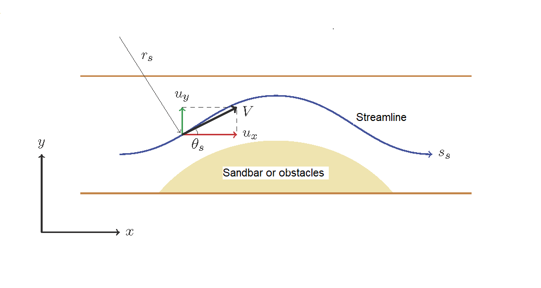
Figure 12.7 : A bending streamline in a straight channel
Now, let us assume that the streamline bends due to sandbars and obstacles, even though the channel is straight, as in Figure 12.7. At this time, centrifugal forces are generated by the bending of the streamline, and as in the uniform bend channel described above, secondary flows are generated. Now we define a new coordinate axis, \(s_s\), along the streamline, as shown in Figure 12.7, and we let \(r_s\) be the radius of curvature generated by the bend. Then, \(r_s\) can be obtained by the following equation.
Where, \(\theta_s\) is an angle between the \(s\) axis and the \(x\) axis and is given by the following equation.
Where, \(u_x\) and \(u_y\) are the velocities in the \(x\) and \(y\) directions, respectively.
Where, \(T=u_y/u_x\). In addition, assuming \(V=\sqrt{u_x^2+u_y^2}\), we have…
Where, \(V=\sqrt{u_s^2+u_n^2}\), Consequently, the curvature of the streamline, \(1/r_s\), is…
The radius of curvature of a streamline can now be determined using only the local flow velocity at each point.
12.2.1.2. For curvilinear coordinates
Next, consider the case of Cartesian curvilinear coordinates, such as the sine-generated-curve of the previous section.
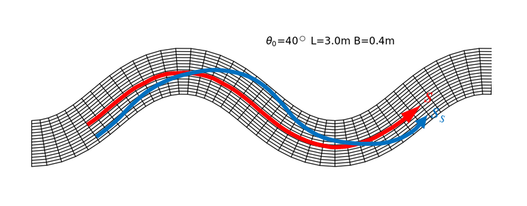
Figure 12.8 : The curvature of a channel and the streamline (1)
As shown in Figure 12.8, we assume the case where the curvature of the streamline and curvature of channel are not on the same line. The red arrow is the coordinate axis along the channel and the blue arrow is the streamline.
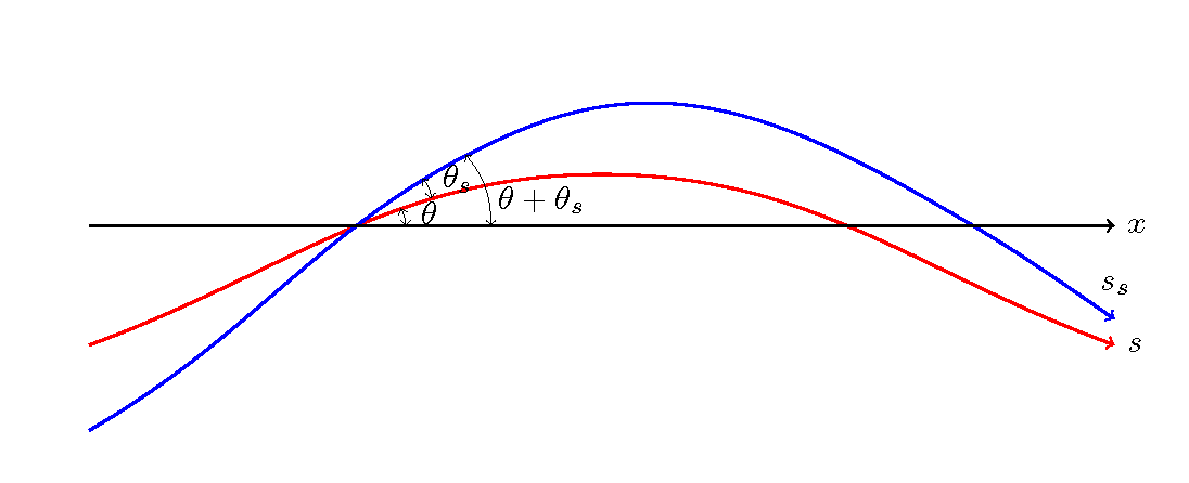
Figure 12.9 : The curvature and angle of a channel and the streamline
As shown in Figure 12.9, assuming that the angle between the coordinate \(s\) axis along the channel and the \(x\) axis is \(\theta_s\) and that the angle between the \(s\) axis and the direction of the streamline is \(\theta_s\), then the angle between the streamline and \(x\) axis is \(\theta+\theta_s\), and the curvature of the streamline is given by the equation below.
Here, for \(\cfrac{\partial \theta}{\partial s}\), such as in the aforementioned Sin-Generated Curve and Kinoshita-Generated Curve, when \(\theta\) is given as a function of \(s\), their differentiations are used. For arbitrary shapes, such as real rivers, the one calculated by the method shown in Calculation of the sinuosity is used. Note that, of course, in the case of a straight line, \(\cfrac{\partial\theta}{\partial s}=0\). For uniform bend flows, such as shown in Figure 12.2, the inverse of the radius of curvature for the chosen concentric circle is used. It should also be noted that, for example, Equation (10.7) gives the curvature of the sine-generated curve, and it gives the curvature of the channel centerline. This means that, depending on the position of the transverse line of the target point, corrections may be required.
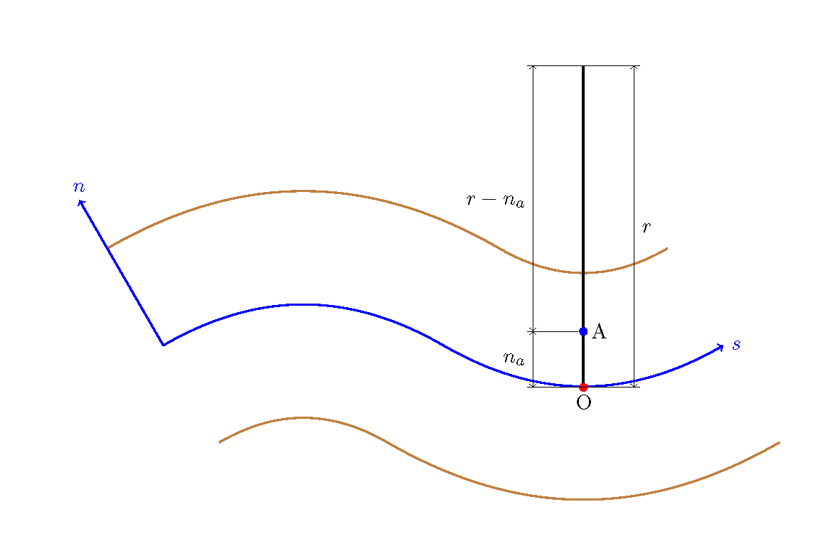
Figure 12.10 : Corrections for the radius of curvature
In the example of Figure 12.10, Point O is at the channel centerline, so no correction for \(r\) is required. However, Point A, which is \(n_a\) close to the left bank from Point O, \(r-n_a\) must be used instead of \(r\).
Regarding \(\cfrac{\partial \theta_s}{\partial s}\), the second term of the right side of Equation (12.17), is a curvature of the component of deviation in the direction of coordinate axis along the channel. Therefore, using \(u_s, u_n\) instead of \(u_x, u_y\) for the derived Equation (12.16) on the \(x-y\) coordinates, we have…
Note that, per the aforementioned calculation, Equation (12.18) gives a curvature of the channel centerline. Therefore, depending on the distance between the calculation point and the centerline, a correction may be required.
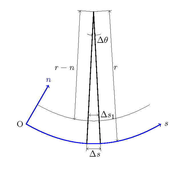
Figure 12.11 : \(\Delta s\) corrections
From Figure 12.11,
Therefore, for Equation (12.18), by replacing \(\cfrac{1}{\partial \theta}\) with \(\cfrac{r}{r-n} \cfrac{1}{\partial \theta}\), we can express the curvature of the streamline at an arbitrary point. That is,
12.2.2. Calculation examples for the curvature of the streamline
12.2.2.1. An example of the sine-generated curve
Let us assume a channel with a sine-generated curve with a gradient \(I\) of 0.001, a wavelength \(L\) of 3 m, a channel width \(B=\) of 0.4 m, and a max. meander angle of \(\theta_0=40^\circ\). Then, using Equation (10.5), we overlay sandbar-like geometry with a max. bar height \(A_p\) of 0.015 m and a phase difference \(\delta\) of 0.2 m. In addition, we give a Manning’s coefficient of roughness \(n_m\) of 0.02, and a discharge \(Q\) of 0.001 m \(^3\)/s.
The 2D flow calculation results are shown as the water depth contour and the depth-averaged velocity vector in Figure 12.12 below.
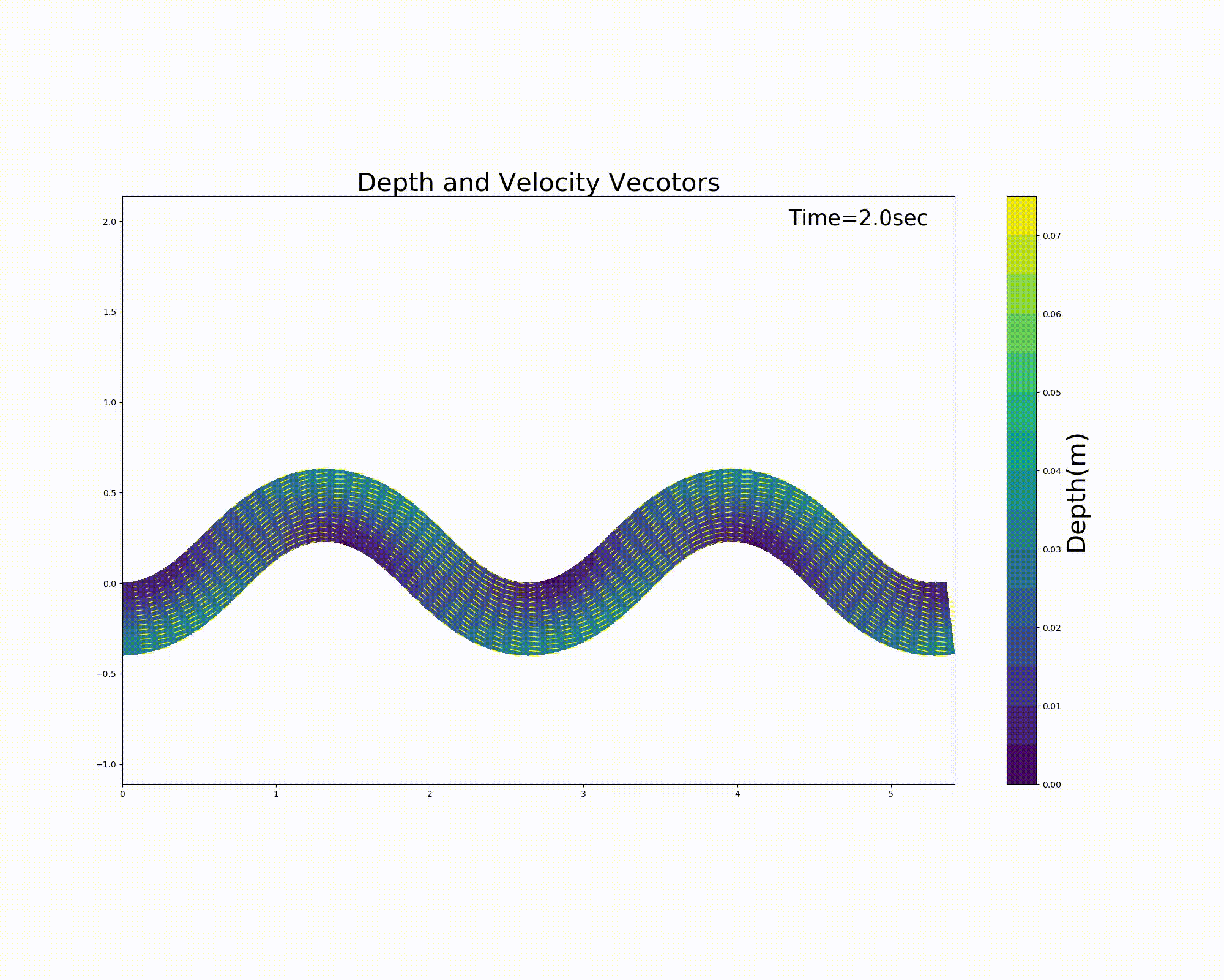
Figure 12.12 : A flow calculation example for the sine-generated curve
The curvature \(1/r\) along the channel centerline and the curvature \(1/r_s\) of the streamline of the depth-averaged velocity along the channel centerline are shown in Figure 12.13 below. Note that \(1/r_s\) is calculated using (12.17) and that \(\cfrac{\partial \theta_s}{\partial s}\) is calculated with Equation (12.18) and falls along the channel centerline. All of the partial differential terms that appear in (12.18) are calculated using central differences.
The streamline curvature becomes slightly unstable immediately after the calculation starts, but then stabilizes. The curvature of the stream is found to be stable with a slight amplitude increase relative to the curvature of the channel and with a slight phase difference in the downstream direction. An increasing curvature means a decreasing radius of curvature. The results are in line with the image of the streamline bend being transmitted downstream relative to the bend of the channel with a phase difference.
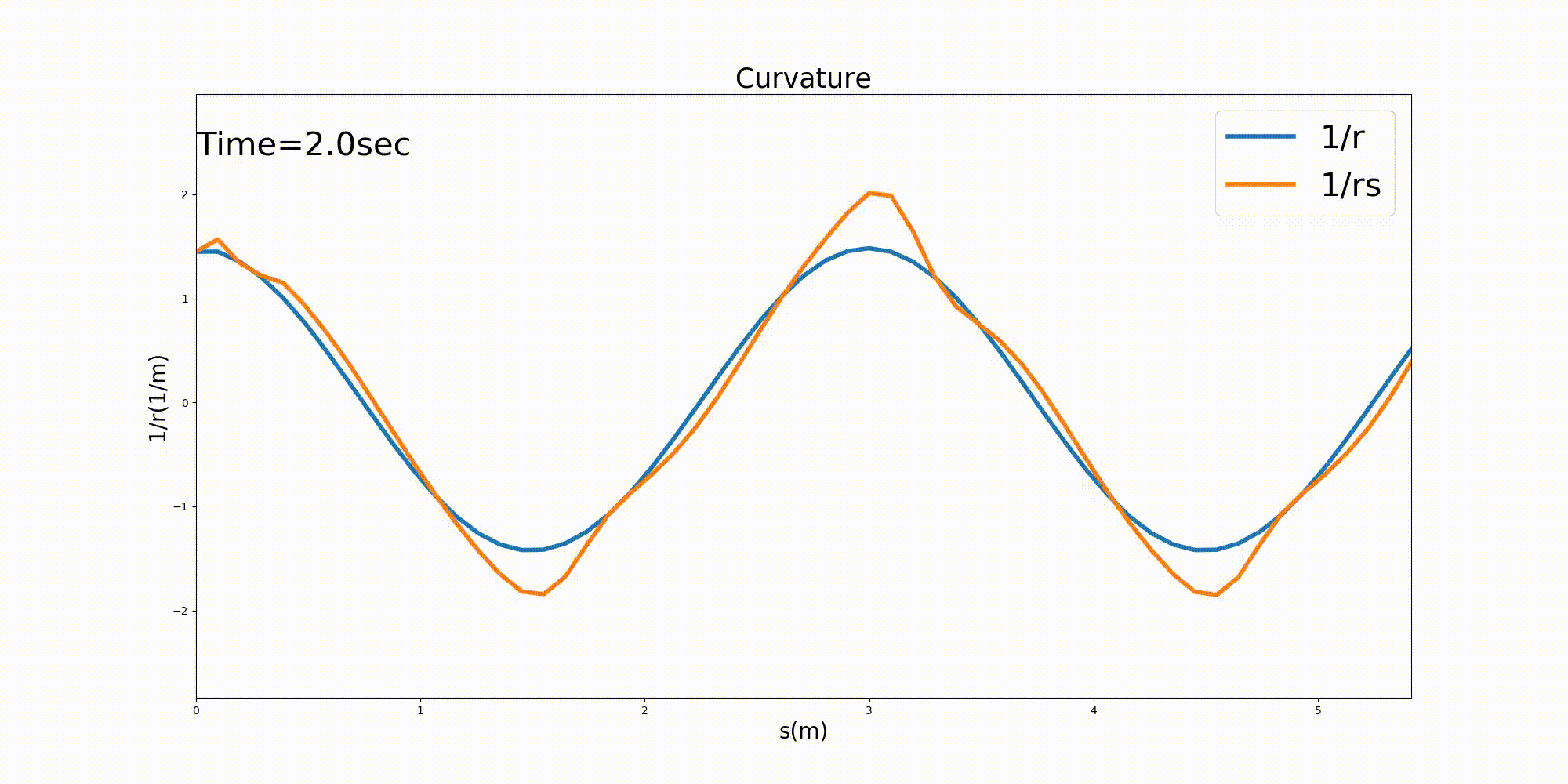
Figure 12.13 : The curvature of a channel and curvature of the streamline with a sine-generated curve
12.2.2.2. A calculation example for a straight channel with a group of spur dikes
In the case of a meandering channel, the curvature of flow along the channel occurs from the beginning. Even in a straight channel, flow bending is generated by obstructions, causing the streamline to curve. For an example, as in Figure 12.14, streamline curvatures also occur when the flow is forced to meander by the installation of spur dikes alternately on the left and right banks of a straight channel.
Figure 12.14 is the result of flow calculation in a straight channel, where, the channel length \(L\) of 4 m, the channel width \(B=\) of 0.4 m, the gradient \(I\) of 0.001, and spur dikes with a length of 12 cm are alternately placed at every 80 cm. Even though the channel is straight, we can see that the flow meanders from left to right because of the spur dikes.
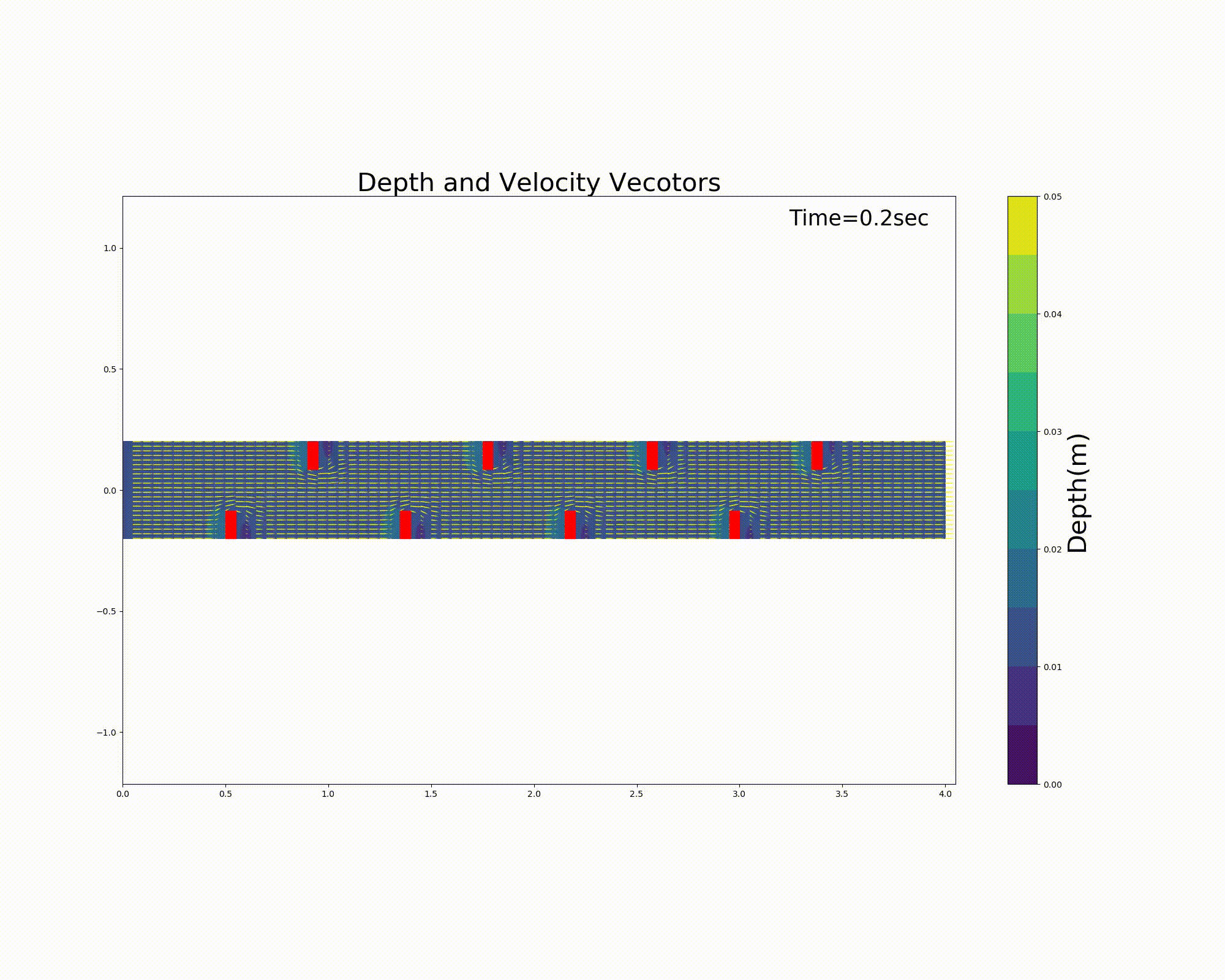
Figure 12.14 : Flow in a straight channel with a group of spur dikes (velocity vectors)
Figure 12.15 is the curvature of the streamline calculated from the above flow field calculations, using the depth-averaged velocity, with the values at the center of the channel plotted longitudinally. The blue line is the curvature of the coordinates obtained from the calculation grid; the orange line is the curvature of the streamline obtained from the flow velocity. Because the channel is straight, the \(s\) axis is straight, so naturally the curvature of the lattice (the blue line) is zero. The curvature of the streamline shows an unsteady distribution to the left and right as the flow meanders. The curvature of the streamline is expected to generate secondary flows and to influence bed deformation in the same way as in the meandering channels mentioned above. For reference, the longitudinal distributions of the discharge, the velocity at the center of the channel, and the water levels along the centerline and along the left and right banks in this case are shown in Figure 12.16.
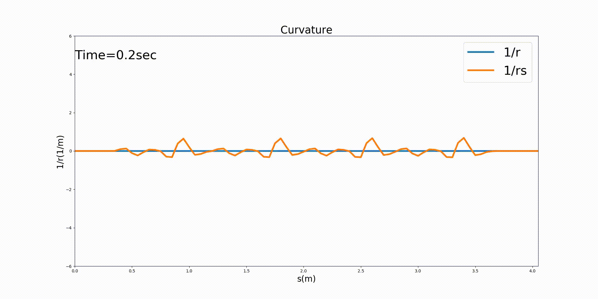
Figure 12.15 : Flow in a straight channel with a group of spur dikes (curvature of the channel and curvature of the streamline)
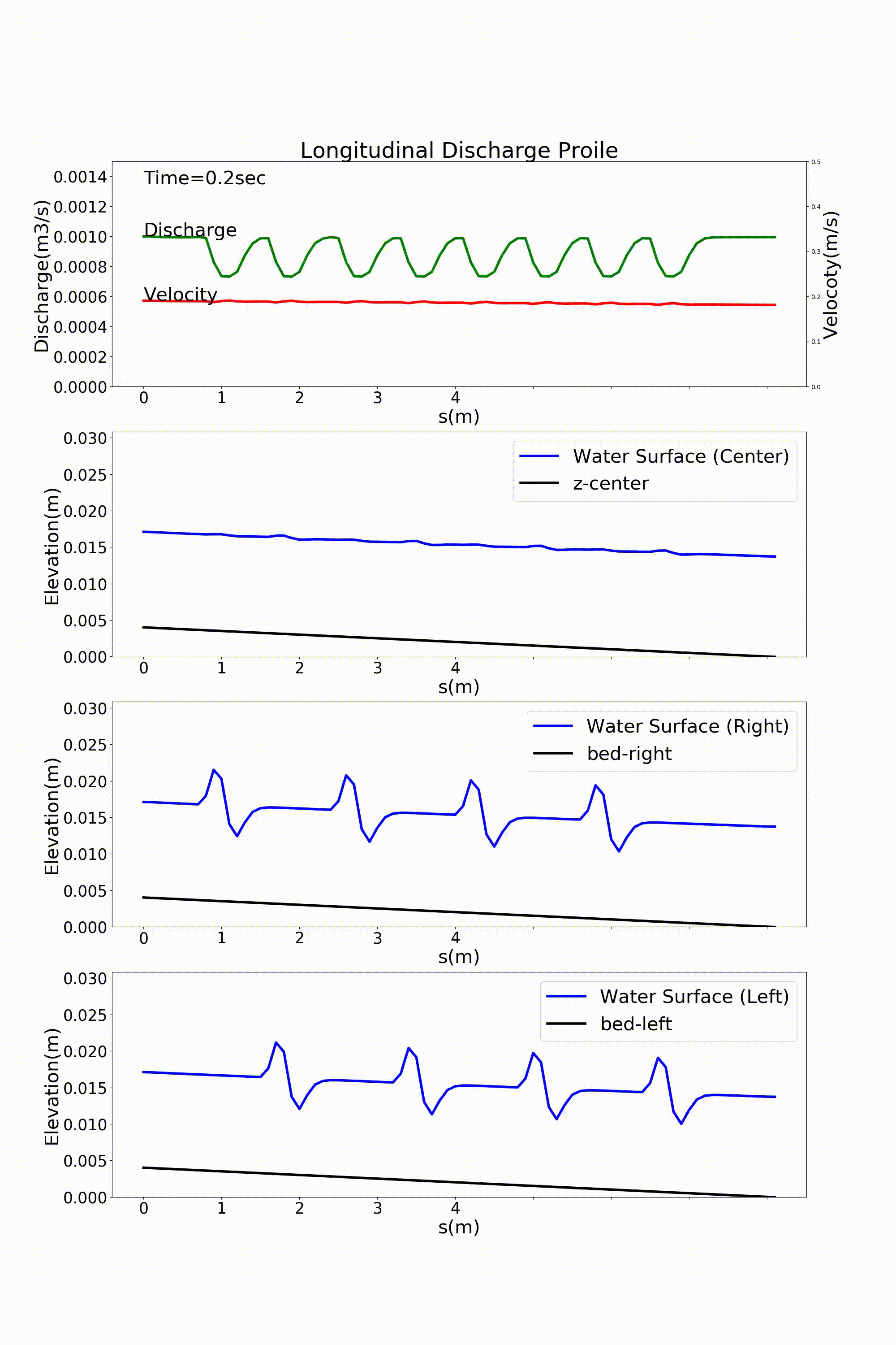
Figure 12.16 : Flow in a straight channel with a group of spur dikes (discharge, flow velocity, longitudinal water surface profile)
Flow with a group of spur dikes can be calculated by using the aforementioned code.
https://github.com/YasuShimizu/Nays2d_sn_python
This is done using “config_groyne.yml” in the same repository, rather than by using “config.yml”. In addition to the channel morphology and hydraulic conditions, the spacing, length, and arrangement of the spur dikes can also be set in the “config.yml” file.
https://github.com/YasuShimizu/Nays2d_sn_python/blob/main/config_groyne.yml
Contents of config_groyne.ym:
j_rep: 0 # periodic boundary conditions (0: no periodic boundary conditions, 1: periodic boundary conditions)

lam : 2.0 # channel wavelength (m)
nx0 : 41 # number of girds/wavelength
ny : 21 # number of girds in the transverse direction (Use an odd number is recommended)
wn : 2 # wave number
chb : 0.4 # channel width (m)
t0_degree : 0 # max. mender deflection angle (degree)
slope: 0.001 # channel gradient
xsize: 20 # transverse scale of the figure for plotting the calculation results

amp : 0.0 # wave height of the initial bed bar (m)
delta : 0. # phase difference of the initial bed bar (m)
beta_0: 0. # rate of channel narrowing at the inner bank
amp_0: 0.0 # bed elevation of the narrowed section (m)

snu_0 : 1e-6 # coefficient of kinematic viscosity
hmin : 0.001 # min. water depth (m)
cw: 0.001 # sidewall friction coefficient
ep_alpha: 1. # eddy viscosity coefficient

qp: 0.001 # discharge (m^3/s)
snm: 0.01 # Manning’s roughness coefficient
g: 9.8 # gravitational acceleration (m/s^2)

j_west: 0 # upstream condition (0: open, 1: closed)
j_east: 0 # downstream condition (0: open, 1: closed)
j_hdown: 1 # water level condition at the downstream end (0: free flow, 1: neutral depth, 2: constant water level)
h_down : 1. # constant water level when j_hdown=2 (m)
j_inih: 2 # initial longitudinal water surface profile (0: straight, 1: uniform flow calculation, 2: non-uniform flow calculation)

alh: 0.6 # relaxation factor for the water level convergence calculation
lmax: 20 # max. number of repetitions of water level convergence calculation at each time step

etime: 60. # calculation end time (sec)
tuk: 0.2 # output interval of calculation results (sec)
dt: 0.01 # calculation time step (sec)
stime: 0. # output start time (sec)

j_obst: 1 # obstacles (0=No, 1=Yes)
jo_type: 2 # method for installing obstacles (1=read from a file, 2=specify the conditions)
jo_method: 4 # 0=No, 1=only right bank, 2=only left bank, 3=right & left banks (alternately), 4=right & left banks (at the same longitudinal locations)
f_dike_pos: 0.5 # position of the first spur dike (m)
dike_dis: 0.8 # interval of spur dikes (m)
dike_length: 0.12 # length of spur dike (m)
dike_thick: 0.02 # width of spur dike (m)
num_dike : 4 # number of spur dikes (per bank)

iskip: 1 # i-direction thinning of vector plots
jskip: 1 # j-direction thinning of vector plots
jscale: 15 # vector scale factor

alpha_upu : 0.05 # relaxation factor of periodic boundary conditions

vcolor : yellow # vector color
rrmax: 6 # max. curvature plot value on an axis (1/m)