13. Calculation of the flow and bed deformation in meandering channels (practical edition)

13.1. Method for calculating 2D sediment transport

13.1.1. The direction of the bottom shear stress resulting from secondary flow

[The information in this section is described in detail in the paper by Nishimura et al. [Ref:40]]

Uniform flow conditions are assumed along the streamline of depth-averaged flow. When Manning’s law is adapted as the law of resistance, then the relationship between the depth-averaged velocity and the bottom shear force is given by Equation (12).

(13.1)\[\tau=\rho g h I_e = {{\rho g n_m^2 V^2}\over{h^{1/3}}}\]

Where, assuming that \(V\) is the resultant composite velocity in the streamline direction, then \(V=\sqrt{u_s^2+u_n^2}\) for the coordinates \(s, n\). The resultant composite non-dimensional tractive force in the streamline direction is given by the following equation.

(13.2)\[\tau_\ast=\cfrac{h I_e}{s d}=\cfrac{n_m^2 V^2}{s d h^{1/3}}\]

By using \(\tau_\ast\), the bedload transport in the streamline direction can be obtained from various bedload transport equations mentioned under sediment transport equations in the previous chapter. Let us denote the bedload transport in the streamline direction as \(q_b\).

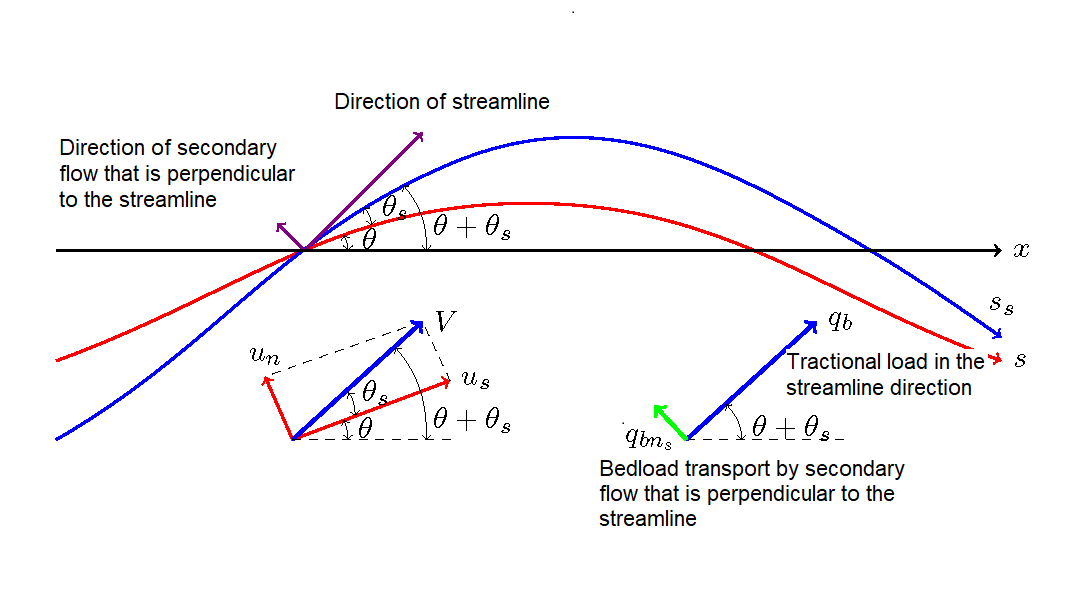
Figure 13.1 : Direction of the bed shear force incorporating secondary flow

The bedload transported by secondary flows can be determined by the following equation, assuming that (12.9) is also valid on a depth-averaged streamline.

(13.3)\[q_{bn_s}= q_b N_\ast \cfrac{h}{r_s}\]

Where, \(q_{bn_s}\) is the bedload transported by secondary flow perpendicular to the streamline, \(N_\ast\) is the secondary flow intensity of Equation (194) (7.0 in general), and \(r_s\) is the radius of curvature of the streamline.

13.1.2. Correction due to the effect of gravity

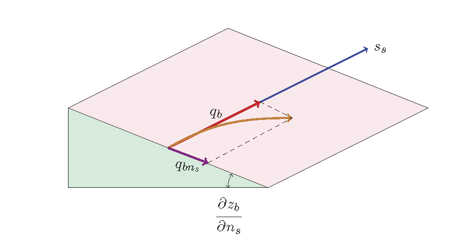
Figure 13.2 : Slope correction of sediment transport

As shown in Figure 13.2, when there is a slope perpendicular to the sediment transport direction, which is the direction of the streamline, then the component of gravity in the slope direction acts on the sediment transport and causes the direction of that transport to bend. For the effects of gravity for a slope in the transverse direction, Hasegawa’s Equation [Ref:27], which takes into account the effects of gravity for the transverse slope together with the aforementioned secondary current effects, is well known.

(13.4)\[q_{bn_s}=q_b \left(N_\ast \cfrac{h}{r_s} -\sqrt{\cfrac{\tau_{\ast c}}{\mu_s \mu_k \tau_\ast}} \cfrac{\partial z_b}{\partial n_s}\right)\]

Where, \(\mu_s, \mu_k\) are the static friction coefficient and the dynamic friction coefficient of sand grains, respectively, \(\tau_{\ast c}\) is the non-dimensional critical tractive force ((8.14)), \(\tau_\ast\) is the non-dimensional tractive force ((8.10)), \(z_b\) is the bed elevation, and \(n_s\) is the direction perpendicular to the streamline of the depth-averaged velocity.

Gravity acts not only in the transverse direction, but also in the longitudinal direction. Watanabe et al. [Ref:39] have proposed a formula that expresses the effects of gravity on the general coordinate system. The effects are shown in the direction of the depth-averaged streamlines and in the direction of the secondary current, which is perpendicular to the streamline, as follows.

(13.5)\[ \begin{align}\begin{aligned}q_{bs_s} & =q_b \left\{ \cfrac{u_{sb}}{\sqrt{{u_{sb}}^2+{u_{nb}}^2}} - \sqrt{\cfrac{\tau_{\ast c}}{\mu_s \mu_k \tau_\ast}} \left( \cfrac{\partial z_b}{\partial s_s} + \cos{\phi}\cfrac{\partial z_b}{\partial n_s} \right) \right\}\\q_{bn_s} & =q_b \left\{ \cfrac{u_{nb}}{\sqrt{{u_{sb}}^2+{u_{nb}}^2}} - \sqrt{\cfrac{\tau_{\ast c}}{\mu_s \mu_k \tau_\ast}} \left( \cfrac{\partial z_b}{\partial n_s} + \cos{\phi}\cfrac{\partial z_b}{\partial s_s} \right) \right\}\end{aligned}\end{align} \]

Where, \(s_s, n_s\) are the coordinate in the direction of the depth-averaged velocity and the axis of coordinate perpendicular to that coordinate, \(q_{bs_s}, q_{bn_s}\), are the unit width bedload transport rates in the \(s_s, n_s\) directions, \(u_{sb}, u_{nb}\) are the bottom flow velocities in the \(s_s, n_s\) directions, and \(\phi\) is an angle between \(s_s\) and \(n_s\). In this section, we assume that \(\cos \phi = 0\). The secondary flow velocity is usually at least one order of magnitude smaller than the main flow velocity and \({u_{nb}}^2 << {u_{sb}}^2\). Therefore,

(13.6)\[\sqrt{{u_{sb}}^2+{u_{nb}}^2} \approx |u_{sb}|\]

Adopting Equation (12.8) for the bed flow velocity in the transverse direction, Equation (13.5) is converted as follows.

(13.7)\[ \begin{align}\begin{aligned}q_{bs_s} & =q_b \left( 1 -\sqrt{\cfrac{\tau_{\ast c}}{\mu_s \mu_k \tau_\ast}} \cfrac{\partial z_b}{\partial s_s} \right)\\q_{bn_s} & =q_b \left( N_\ast \cfrac{h}{r_s} -\sqrt{\cfrac{\tau_{\ast c}}{\mu_s \mu_k \tau_\ast}} \cfrac{\partial z_b}{\partial n_s} \right)\end{aligned}\end{align} \]

Regarding \(\cfrac{\partial z_b}{\partial s_s}\) and \(\cfrac{\partial z_b}{\partial n_s}\)，

(13.8)\[ \begin{align}\begin{aligned}\cfrac{\partial z_b}{\partial s_s} =\cfrac{\partial s}{\partial s_s} \cfrac{\partial z_b}{\partial s}+ \cfrac{\partial n}{\partial s_s} \cfrac{\partial z_b}{\partial n} =\cfrac{u_s}{V}\cfrac{\partial z_b}{\partial s}+ \cfrac{u_n}{V}\cfrac{\partial z_b}{\partial n}\\\cfrac{\partial z_b}{\partial n_s} =\cfrac{\partial s}{\partial n_s} \cfrac{\partial z_b}{\partial s}+ \cfrac{\partial n}{\partial n_s} \cfrac{\partial z_b}{\partial n} =-\cfrac{u_n}{V}\cfrac{\partial z_b}{\partial s}+ \cfrac{u_s}{V}\cfrac{\partial z_b}{\partial n}\end{aligned}\end{align} \]

When bed deformation calculations are made on the \(s,n\) coordinates, we need to determine sediment transport, \(q_{bs}, q_{bn}\), in the directions of the \(s,n\) axes. They are calculated from the following equation by using \(q_{bs_s}, q_{bn_s}\) given by Equation (13.7).

(13.9)\[ \begin{align}\begin{aligned}q_{bs}=q_{bs_s} \cos\theta_s - q_{bn_s} \sin\theta_s = q_{bs_s} \cfrac{u_s}{V}-q_{bn_s}\cfrac{u_n}{V}\\q_{bn}=q_{bs_s} \sin\theta_s + q_{bn_s} \cos\theta_s = q_{bs_s} \cfrac{u_n}{V}+q_{bn_s}\cfrac{u_s}{V}\end{aligned}\end{align} \]

Where, \(\cos \theta_s = \cfrac{u_s}{V}\), \(\sin \theta_s = \cfrac{u_n}{V}\) (Figure 13.1 refers to the bottom left figure.)

Consequently, based on equations (13.7), (13.8), and (13.9), we have…

(13.10)\[ \begin{align}\begin{aligned}q_{bs} & =q_b \left\{ \cfrac{1}{V} (u_s - u_n N_\ast \cfrac{h}{r_s}) -\sqrt{\cfrac{\tau_{\ast c}}{\mu_s \mu_k \tau_\ast}} \cfrac{\partial z_b}{\partial s} \right\}\\q_{bn} & =q_b \left\{ \cfrac{1}{V} (u_n + u_s N_\ast \cfrac{h}{r_s}) -\sqrt{\cfrac{\tau_{\ast c}}{\mu_s \mu_k \tau_\ast}} \cfrac{\partial z_b}{\partial n} \right\}\end{aligned}\end{align} \]

13.1.3. The introduction of a slope failure model

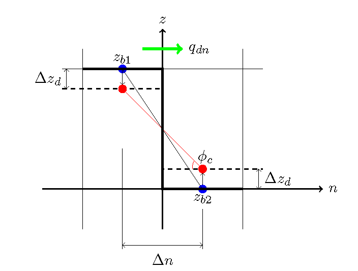
Figure 13.3 : The slope failure model

As shown in Figure 13.3, let us assume that the slope angle between adjacent grids in a certain part of the cross section exceeds the angle of repose, \(\phi_c\). In this case, even if there is no sediment transport, implicit sediment transport occurs when slope failures are considered to occur. Now, we set the bed heights of the two adjacent points as \(z_{b1}, z_{b2}\) and, the distance between them as \(\Delta n\). This gives us…

(13.11)\[-\cfrac{\partial z_b}{\partial n} = \cfrac{z_{b1}-z_{b2}}{\Delta n} > \tan \phi_c\]

At this time, from the difference expression of the continuity equation of sediment transport, we have…

(13.12)\[(q_{dn}-0)\Delta t=\Delta z_d \Delta n (1-\lambda)\]

Where, \(q_{dn}\) is the slope failure-derived sediment flux, converted to unit width sediment transport rate, \(\Delta t\) is the time interval for numerical calculations, \(\Delta z_d\) is the ground level reduction in the upper slope from slope failure (= the ground elevation increase in the lower slope due to sediment supplied by the slope failure), \(\Delta n\) is the distance between the two points, and \(\lambda\) is the void ratio. Slope failure causes the slope gradient between the two points to moderate to the angle of repose, i.e., the gradient after the change in ground level is the angle of repose. This gives us…

(13.13)\[\cfrac{(z_{b1}-\Delta z_d)-(z_{b2}+\Delta z_d)}{\Delta n}= \tan \phi_c\]

Consequently, (13.12) and (13.13) give us

(13.14)\[q_{dn}=-\left( \cfrac{\partial z_b}{\partial n}+\tan \phi_c \right) \cfrac{(1-\lambda)}{2\Delta t} \Delta n^2\]

Similarly, for

(13.15)\[\cfrac{\partial z_b}{\partial n} = \cfrac{z_{b2}-z_{b1}}{\Delta n} > \tan \phi_c\]

(13.16)\[q_{dn}=-\left( \cfrac{\partial z_b}{\partial n}-\tan \phi_c \right) \cfrac{(1-\lambda)}{2\Delta t} \Delta n^2\]

We rewrite these as a single equation. Then, we have….

(13.17)\[\left|\cfrac{\partial z_b}{\partial n} \right| > \tan\phi_c \hspace{5mm} \mbox{when} \hspace{5mm} q_{dn}=-\left\{ \cfrac{\partial z_b}{\partial n} + \mbox{sign} \left(\cfrac{\partial z_b}{\partial n} \right) \tan \phi_c \right\} \cfrac{(1-\lambda)}{2\Delta t} \Delta n^2\]

Similarly for the \(s\) axis direction…

(13.18)\[\left|\cfrac{\partial z_b}{\partial s} \right| > \tan\phi_c \hspace{5mm} \mbox{when} \hspace{5mm} q_{ds}=-\left\{ \cfrac{\partial z_b}{\partial s} + \mbox{sign} \left(\cfrac{\partial z_b}{\partial s} \right) \tan \phi_c \right\} \cfrac{(1-\lambda)}{2\Delta t} \Delta s^2\]

Where, \(q_{ds}\) is the converted value of the slope failure sediment amount in the \(s\) axis direction. When you take into account the slope failure, the slope failure sediment amounts given by equations (13.17) and (13.18) are added to Equation (13.10).

13.2. The equation of continuity for sediment transport on a 2D riverbed

The equation of continuity for the coordinates \(s,n\) (Cartesian curvilinear coordinates) is converted into the following equation by replacing the water flux part in the equation of continuity for water, (129), which is derived from Derivation of the equation of continuity on the s-n coordinates (alternative solution), with the sediment transport flux and by taking the void ratio into account.

(13.19)\[\cfrac{\partial z_b}{\partial t} + \cfrac{1}{1-\lambda}\left( \cfrac{\partial q_{bs}}{\partial s}+ \cfrac{1}{r}\cfrac{\partial(r q_{bn})}{\partial n} \right)=0\]

Where, \(q_{bs}, q_{bn}\) are the unit width sediment transport rates in the directions of \(s, n\), respectively. Similar to (11.4), the temporal changes in bed elevation are given by the following equation.

(13.20)\[ \begin{align}\begin{aligned}\cfrac{\partial z_b}{\partial t}A_x(i,j) = \cfrac{1}{1-\lambda} \left\{ q_{bs}(i-1,j)\Delta n(i-1,j)-q_{bs}(i,j)\Delta n(i,j) \right.\\\left. + q_{bn}(i,j-1)\Delta s(i,j-1)-q_{bn}(i,j)\Delta s(i,j) \right\}\end{aligned}\end{align} \]

13.3. Procedure for 2D bed deformation calculation

The procedure for calculating the riverbed deformation is as follows.

1. Set the calculation girds and the initial bed elevation.

2. Calculate the curvature (\(1/r\)) along the grid [Equation (10.12)].

3. Set the calculation conditions (boundary conditions, initial conditions and hydraulic variables).

4. Time \(t=0\)

5. Calculate the water velocity and the water depth by using the calculation method shown by [Calculation of 2D flow in meandering channels (practical edition)]

6. Calculate the curvature of the streamline (\(1/r_s\)) [Equations (12.17), \(\sim\) and (12.20)] d

7. Calculate the bed shear force and the total sediment transport.

8. Calculate the sediment transport in the directions of \(s, n\) [Equation (13.10)].

9. When slope failure is taking into account, use Equation (13.18) and combine the calculation results with the sediment transport in the directions of \(s, n\).

10. Calculate the bed deformation [Equation (13.20)].

11. Update the time \(t=t+\Delta t\)

12. Return to “5.” and repeat the calculations (until a preset time has elapsed).

13.4. Calculation code and calculation results

The calculation codes for flow in a 2D meandering channel and for bed deformation following the explanation thus far are given here.

https://github.com/YasuShimizu/Nays2d_Bed_Deformation

Hasegawa [Ref:27] conducted movable bed experiment (Me-2) shown in Figure 13.4. Figure 13.5 is an example of a reproduction that uses this code for the movable bed experiment (Me-2). The calculation results seem to closely reproduce the experimental results.

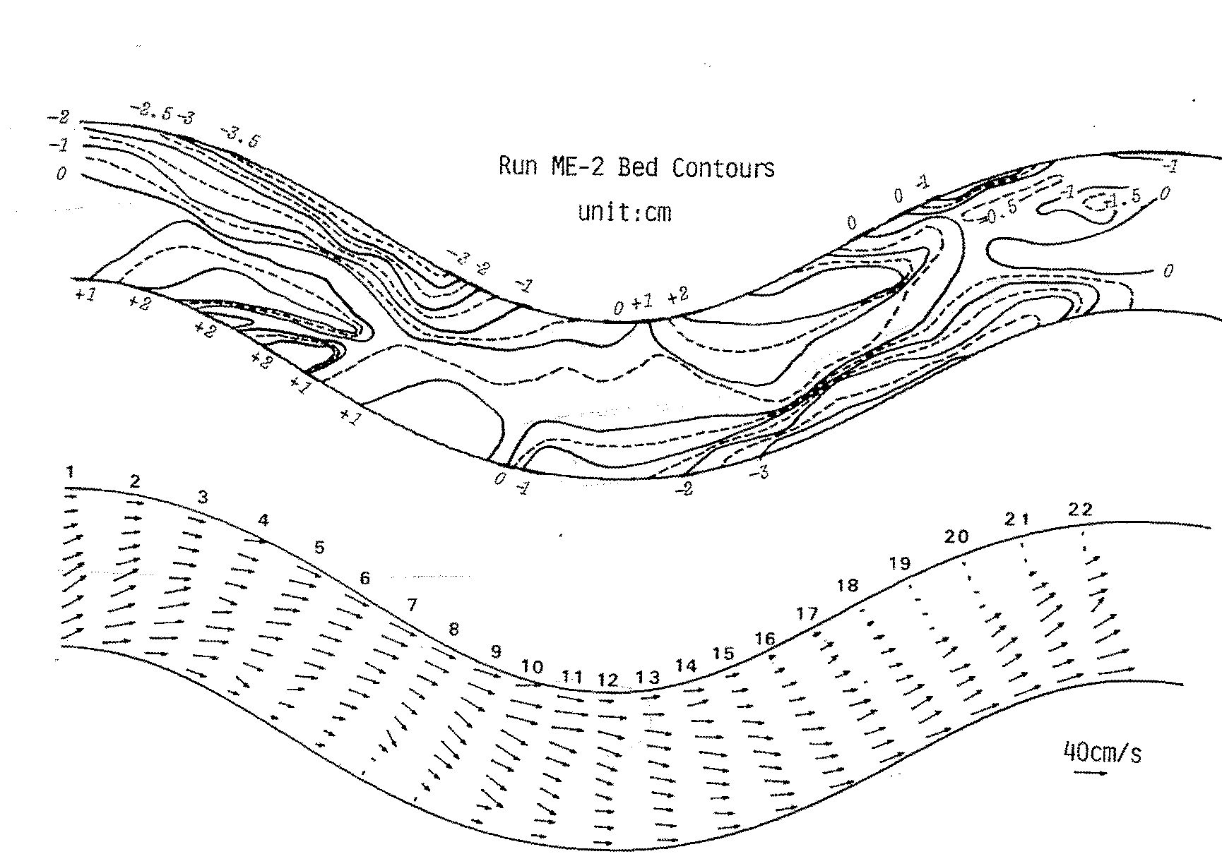
Figure 13.4 : Experimental results of Hasegawa (1986) [Ref:27]_(Me-2)

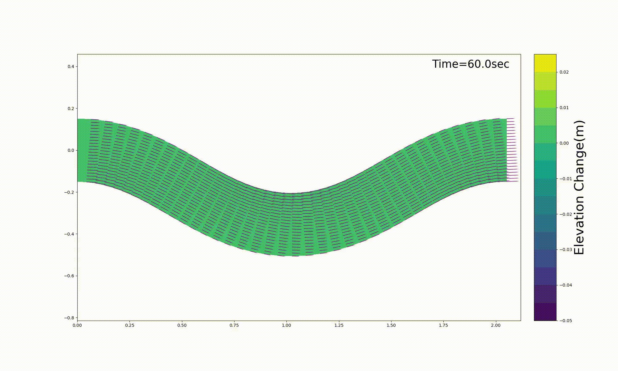
Figure 13.5 : Reproduction calculation for the experimental results of Hasegawa (1986) [Ref:27]

All the parameters and calculation conditions used in the examples of Figure 13.5 are described in a file named “me-2.yml” in the GitHub Repository, where the above source code is available. When executing the calculation, these conditions are read and then the calculation proceeds.

https://github.com/YasuShimizu/Nays2d_Bed_Deformation/blob/main/me-2.yml

Each parameter is described next to each item. In this text, I do not discuss all of the parameters. You can see what the parameter means by comparing it with the source code. Basically, using default values for the parameters should be fine.

The contents of “me-2.yml” are as follows.

j_rep: 1 # periodic boundary conditions (0: no periodic boundary conditions, 1: periodic boundary conditions)

lam : 2.2 # channel wavelength (m) nx0 : 41 # number of girds/wavelength ny : 21 # number of girds in the transverse direction (Use an odd number is recommended) wn : 1 # wave number chb : 0.3 # channel width (m) t0_degree : -30 # max. mender deflection angle (degree) slope: 0.00333 # channel gradient xsize: 20 # transverse scale of the figure for plotting the calculation results

amp : 0.0 # wave height of the initial bed bar (m) delta : 0. # phase difference of the initial bed bar (m) beta_0: 0. # rate of channel narrowing at the inner bank amp_0: 0.0 # bed elevation of the narrowed section (m)

snu_0 : 1e-6 # coefficient of kinematic viscosity hmin : 0.0001 # min. water depth (m) vmin : 0.0001 # min. water velocity (m) cw: 0.001 # sidewall friction coefficient ep_alpha: 1. # eddy viscosity coefficient

qp: 0.00187 # discharge (m^3/s) snm: 0.021 # Manning’s roughness coefficient g: 9.8 # gravitational acceleration (m/s^2) diam: 0.00043 # average grain diameter of bed materials (m) slambda: 0.4 # void ratio musk: 0.1 # μs × μk “static friction coefficient” × “dynamic friction coefficient” nsta: 7.0 # secondary flow intensity

j_west: 0 # upstream condition (0: open, 1: closed) j_east: 0 # downstream condition (0: open, 1: closed) j_hdown: 1 # water level condition at the downstream end (0: free flow, 1: neutral depth, 2: constant water level) h_down : 1. # constant water level when j_hdown=2 (m) j_inih: 2 # initial longitudinal water surface profile (0: straight, 1: uniform flow calculation, 2: non-uniform flow calculation)

alh: 0.7 # relaxation factor for the water level convergence calculation lmax: 10 # max. number of repetitions of water level convergence calculation at each time step

etime: 2400. # calculation end time (sec) tuk: 10. # output interval of calculation results (sec) dt: 0.002 # calculation time step (sec) stime: 0. # output start time (sec) bstime: 60. # bed deformation start time (sec)

j_obst: 0 # obstacles (0=No, 1=Yes) jo_type: 2 # method for installing obstacles (1=read from a file, 2=specify the conditions) jo_method: 4 # 0=No, 1=only right bank, 2=only left bank, 3=right & left banks (alternately), 4=right & left banks (at the same longitudinal locations) f_dike_pos: 0.8 # position of the first spur dike (m) dike_dis: 0.8 # interval of spur dikes (m) dike_length: 0.1 # length of spur dike (m) dike_thick: 0.02 # width of spur dike (m) num_dike : 3 # number of spur dikes (per bank)

iskip: 1 # i-direction thinning of vector plots jskip: 1 # j-direction thinning of vector plots jscale: 10 # flow vector scale factor

alpha_upu : 0.1 # relaxation factor of periodic boundary conditions

vcolor : yellow # vector color rrmax: 1 # max. curvature plot value on an axis (1/m)

dz_min: -0.05 # min. bed deformation contour plot (m) dz_max: 0.03 # max. bed deformation contour plot (m) dz_step: 0.005 # step of above contour

The main code is in “main.py”, which executes other functions to define the grid, calculate the flow and the riverbed deformation, and create various plots and animations. (In Python, everything is called a function, not a subroutine. In fact, the functions work as subroutines.) Various hourly plots will be rendered and saved in the folders [png], [ping_q], [ping_r], [sed] and [bed]. Please create these folders in advance.

After the calculation starts, the following diagrams are created and saved in each folder.

1. [ini_contour.png] A contour diagram of the initial bed elevation (flat by default)

2. [curvature.png] A longitudinal curvature diagram of the calculated grid coordinates along the channel centerline

3. [longitudinal_prof.png] Longitudinal diagrams of the initial riverbed and the initial water surface profile

4. [grid.png] A planar diagram of the calculation grids

After this, the calculation starts, and the following diagrams are created and saved in each folder for each [tuk calculation result output interval (sec)] that is specified in the “yml file”.

1. [png] folder: “png” files of the water depth contour and of mean velocity vector diagrams

2. [ping_q] folder: the discharge, depth-averaged velocity at the channel center, and longitudinal diagrams of the bed and water level along the channel center, near the left bank, and near the right bank.

3. [ping_r] folder: calculation grids and the curvature of the streamline along the channel center and the longitudinal distributions of the curvature of the streamlines near the right bank and the left bank

4. [sed] folder: a vector diagram of the bedload transport

5. [bed] folder: a contour diagram of the bed elevation (the amount of change from the initial bed) and vector diagrams of water depth and velocity

Once all of the calculations have been completed, the following animations in gif and mp4 formats are created using still images that have been created at each output time and that have been saved in each of the above folders.

1. [vec.gif] [vec.mp4] Animations of the water depth contour and of mean flow velocity vector diagrams that change over time

2. [longi.gif] [longi.mp4] Animations of longitudinal diagrams of discharge, flow velocity, channel centerline and bed and water levels

3. [radius.gif] [radius.mp4] Animations of grids and of the curvature of the streamline

4. [sed.gif] [sed.mp4] Animations of the sediment transport vector

5. [bed.gif] [bed.mp4] Animations of variations in the bed elevation contour and of vector diagrams of the water depth and velocity

The calculated results for bed deformation shown in Figure 13.5 are pasted directly from the above [bed.gif].