11. Calculation of 2D flow in meandering channels (practical edition)

11.1. Basic equations

Let us assume that the \(s\) axis is the axis in the flow direction and that the \(n\) axis is the axis in the cross-sectional direction. When we assume that the \(s\) axis freely meanders from left to right along the flow channel, and that the \(n\) axis is always perpendicular to the \(s\) axis, then, the coordinates are named as Cartesian curvilinear coordinates. Or, sometimes the coordinates are simply called a \(s-n\) coordinate system. Strictly speaking, it is a \(s-n\) Cartesian curvilinear coordinate system.

The derivations for the basic formulas for flow calculation for the \(s-n\) coordinate system are shown in Appendix II (Appendix II (Basic equations for 2D flow in the s-n coordinates)). Here, we show only the calculation results.

(11.1)\[\cfrac{\partial h}{\partial t} +\cfrac{\partial(hu_s)}{\partial s} +\cfrac{1}{r}\cfrac{\partial(rhu_n)}{\partial n} =0\]

(11.2)\[ \begin{align}\begin{aligned}{{\partial u_s}\over{\partial t}} +u_s{{\partial u_s}\over{\partial s}} +u_n{{\partial u_s}\over{\partial n}} -{{u_s u_n}\over{r}}= \hspace{4.5cm}\\-g\cfrac{\partial H}{\partial s} -{{g n_m^2 u_s \sqrt{u_s^2+u_n^2}}\over h^{4/3}} +\cfrac{\partial}{\partial s}\left(\nu_t\cfrac{\partial u_s}{\partial s}\right) +\cfrac{\partial}{\partial n}\left(\nu_t\cfrac{\partial u_s}{\partial n}\right) +\cfrac{\nu_t}{r}\cfrac{\partial u_s}{\partial n}\end{aligned}\end{align} \]

(11.3)\[ \begin{align}\begin{aligned}{{\partial u_n}\over{\partial t}} +u_s{{\partial u_n}\over{\partial s}} +u_n{{\partial u_n}\over{\partial n}} +{{u_s^2}\over{r}}= \hspace{4.5cm}\\-g\cfrac{\partial H}{\partial n} -{{g n_m^2 u_n \sqrt{u_s^2+u_n^2}}\over h^{4/3}} +\cfrac{\partial}{\partial s}\left(\nu_t \cfrac{\partial u_n}{\partial s}\right) +\cfrac{\partial}{\partial n}\left(\nu_t\cfrac{\partial u_n}{\partial n}\right) +\cfrac{\nu_t}{r}\cfrac{\partial u_n}{\partial n}\end{aligned}\end{align} \]

Where, \(u_s, u_n\) are the depth-averaged velocities in the \(s, n\) directions, \(h, H\) are the water depth and the water elevation, \(r\) is the radius of curvature for coordinate along the \(s\) axis (for the left curve from upstream to downstream, \(r>0\)), \(n_m\) is the Manning’s coefficient of roughness, and \(\nu_t\) is the eddy-viscosity coefficient.

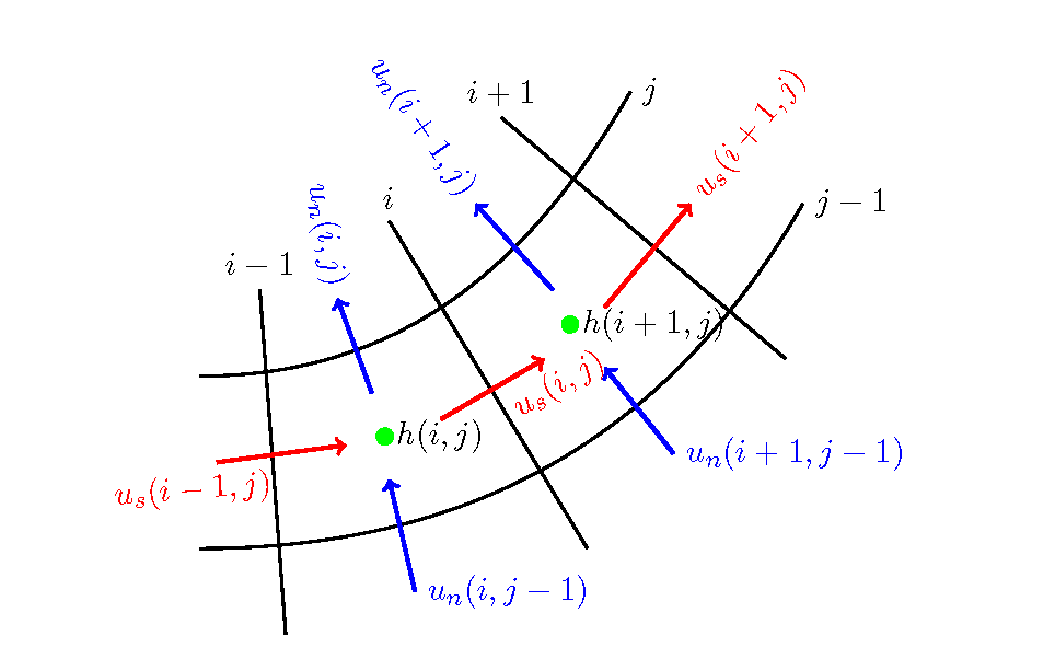
Figure 11.1 : Locations of calculation points for \(u_s, u_n\)

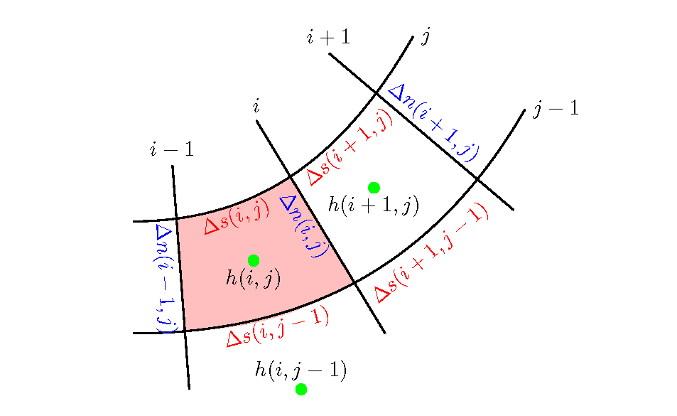
Figure 11.2 : :math: Locations of calculation points for \(\Delta s, \Delta n\) and \(h\)

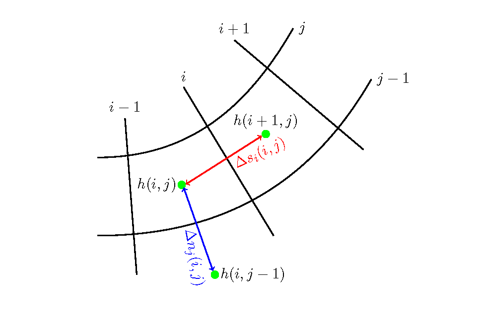
Figure 11.3 : Locations of \(\Delta s_i, \Delta n_j\)

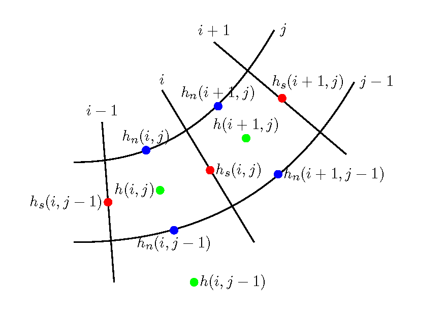
Figure 11.4 : Locations of \(h_s, h_n\)

Based on the locations of the valuables, the equation of continuity, Equation (11.1), for example, can be expressed by the following equation while considering the flux balance of the infinitesimal element (pink part of Figure 11.2), in the same way as in Equation (121).

(11.4)\[ \begin{align}\begin{aligned}\cfrac{\partial h}{\partial t}A_x(i,j) = \hspace{15cm}\\q_s(i-1,j)\Delta n(i-1,j)-q_s(i,j)\Delta n(i,j)+ q_n(i,j-1)\Delta s(i,j-1)-q_n(i,j)\Delta s(i,j)\end{aligned}\end{align} \]

Where, \(q_s, q_n\) are the unit width discharge flux in the \(s, n\) directions. (The unit width discharge and the arrangement of calculation points are the same as \(u_s, u_n\) in Figure 11.1). \(A_x(i,j)\) is the area of the infinitesimal element, which is approximately given by the following.

(11.5)\[A_x(i,j)=\cfrac{\Delta s(i,j)+\Delta s(i,j-1)}{2}\cdot \cfrac{\Delta n(i,j)+\Delta n(i-1,j)}{2}\]

Also,

(11.6)\[ \begin{align}\begin{aligned}q_s(i,j)=u_s(i,j) h_s(i,j)=u_s(i,j)\cfrac{h(i,j)+h(i+1,j)}{2}\\q_n(i,j)=u_n(i,j) h_n(i,j)=u_s(i,j)\cfrac{h(i,j)+h(i,j+1)}{2}\end{aligned}\end{align} \]

11.2. Calculation method

In principle, the calculation method is the same as that for the 2D Cartesian coordinate system that is explained at 2-dimensional unsteady flow with free water surface. By substituting \(\Delta x, \Delta y\), which incorporates local sinuosity changes in the channel shown by Figure 11.2, for \(\Delta s, \Delta n\), which we used in calculating the Cartesian coordinates, we can make calculations in almost the same way as shown in 2-dimensional unsteady flow with free water surface.

When we compare the forms of Equation (11.2) and Equation (11.3) (the equations of motion in the \(s, n\) directions) to those of Equation (7.2) and Equation (7.3) (the equations of motion in the \(x, y\) directions of the Cartesian coordinate system), we can see that the left side of the former has terms that are not in the later, such as \(-\cfrac{u_s u_n}{r}\) and \(\cfrac{u_s^2}{r}\). These terms show additional accelerations associated with the bending of the channel. They need to be addressed in the non-advection phase.

Specifically, what we do is substitute Equation (7.9) and Equation (7.13) with the following.

(11.7)\[{{\partial u_s}\over{\partial t}}= -g\cfrac{\partial H}{\partial s} -{{g n_m^2 u_s \sqrt{u_s^2+u_n^2}}\over h^{4/3}} +{{u_s u_n}\over{r}}\]

(11.8)\[{{\partial u_n}\over{\partial t}}= -g\cfrac{\partial H}{\partial n} -{{g n_m^2 u_n \sqrt{u_s^2+u_n^2}}\over h^{4/3}} -{{u_s^2}\over{r}}\]

As a result, equations corresponding to Equation (7.18) and Equation (7.19) in the non-advection phase I are as follows.

(11.9)\[\overline{u_s}= u_s^n +\Delta t\left\{ - g{{\partial \overline{h}}\over{\partial s}} - g{{\partial \eta}\over{\partial s}} - g{{n_m^2 \overline{u_s}\sqrt{\overline{u_s}^2 +\overline{u_{ns}}^2}} \over{\overline{h_s}^{4/3}}} +{{\overline{u_s}\; \overline{u_{ns}}}\over{r_s}}\right\}\]

(11.10)\[\overline{u_n}= u_n^n+\Delta t\left\{- g{{\partial \overline{h}}\over{\partial n}} - g{{\partial \eta}\over{\partial n}} - g{{n_m^2 \overline{u_n}\sqrt{\overline{u_{sn}}^2 +\overline{u_n}^2}} \over{\overline{h_n}^{4/3}}} -{{\overline{u_{sn}}^2}\over{r_n}} \right\}\]

Where, parameters with an over bar are values in the non-advection phase I. These parameters are obtained as the simultaneous solutions to the equation of continuity of (11.4) and to the equation above by calculation repetitions. \(h_s, u_{ns}\) are the water depth and the flow velocity in the direction of the \(n\) axis at the calculation points \(u_s\), \(h_n, u_{sn}\) are the water depth and the flow velocity in the direction of the \(s\) axis at the calculation points \(u_n\). \(u_{ns}, u_{sn}\) are given by the following equations.

(11.11)\[ \begin{align}\begin{aligned}u_{ns}(i,j)=\cfrac{u_n(i,j)+u_n(i+1,j)+u_n(i,j-1)+u_n(i+1,j-1)}{4}\\u_{sn}(i,j)=\cfrac{u_s(i,j)+u_s(i,j+1)+u_s(i-1,j)+u_s(i-1,j+1)}{4}\end{aligned}\end{align} \]

\(r_s\) and \(r_n\) are the radii of curvature at calculation points \(u_s\) and u_n, respectively. Now, when we define the radius of curvature along the \(s\) axis at the calculation grid point using (10.12), we assume a curvature that is the reciprocal of the radius of curvature, as follows.

(11.12)\[\rho_r(i,j) = \cfrac{1}{r(i,j)}\]

Then, Equation \(r_s, r_n\) is transformed as follows.

(11.13)\[ \begin{align}\begin{aligned}\cfrac{1}{r_s(i,j)}=\cfrac{\rho_r(i,j)+\rho_r(i,j-1)}{2}\\\cfrac{1}{r_n(i,j)}=\cfrac{\rho_r(i,j)+\rho_r(i-1,j)}{2}\end{aligned}\end{align} \]

Because other parts of the calculation are exactly the same as the aforementioned 2-dimensional unsteady flow with free water surface, we omit them here.

11.3. Dry Bed (calculation point with no water)

When a bed morphology with sandbars, such as was introduced in a previous section [Giving a “bar and pool” geometry to the bed], is given as a condition of calculation and when the bed rises due to the influence of sandbars in bed deformation calculations (cases to be introduced later), then the water depth calculated by the equation of continuity, Equation (11.4), becomes zero, i.e., calculation cells with no water occur. In a real calculation, the calculation of (11.4) gives a negative water depth in some instances. In such a case, the water depth is set as zero for convenience. The equations of motion, Equation (11.2) and Equation (11.3), include the water depth, \(h\), in the denominator of the second term on the right side. When the water depth is zero or is approaching to zero, a calculation divergence occurs. When the water depth is zero, the flow velocity also should be zero. However, when we use a staggered grid, there may be cases in which the flow velocity calculated for the edges of the cell is not zero, even when the water depth at the center of the cell is zero. Therefore, we need to pay special attention to such cases. A calculation point with a water depth of zero is called “a dry bed,” and it requires a special calculation method.

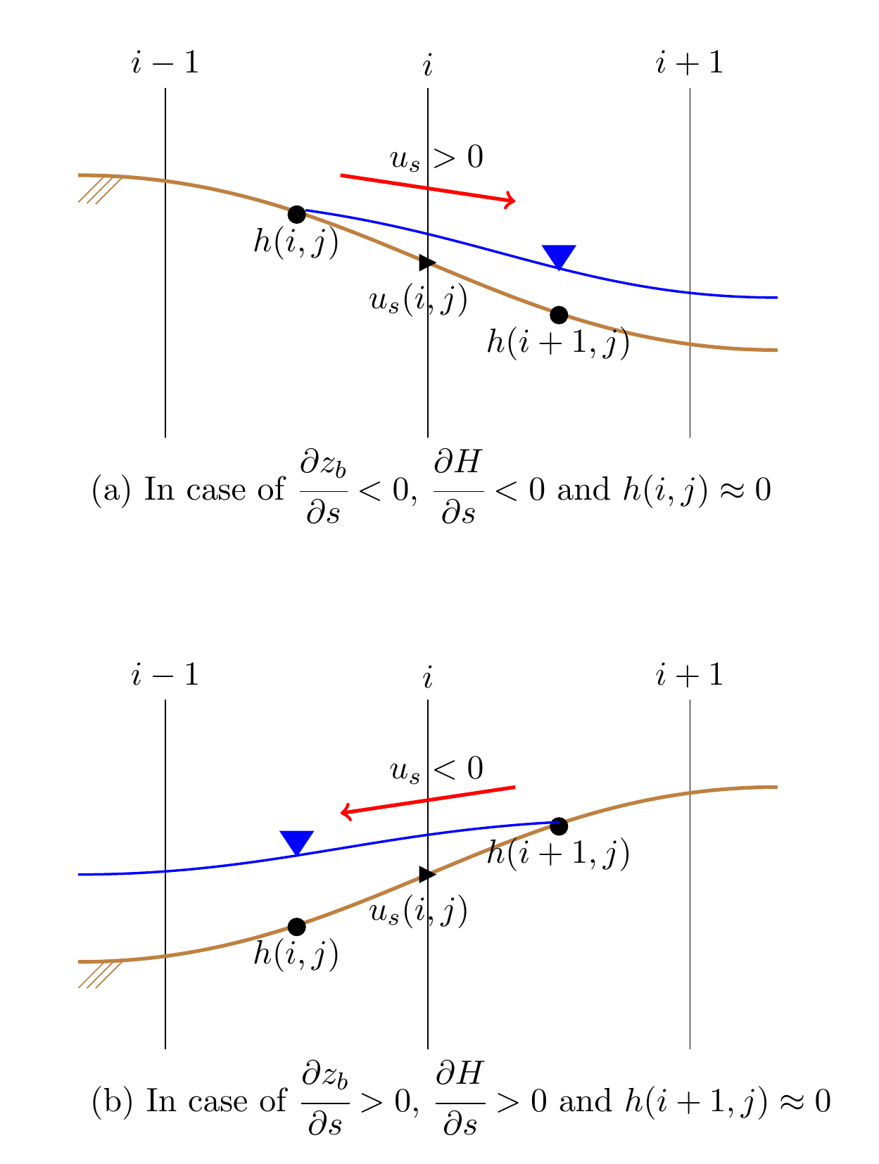
Figure 11.5 : Dry bed calculation method

For example, when calculating \(u_s\), we need the water levels immediately upstream and immediately downstream of the calculation point (the water surface gradient). When the water level either immediately upstream or immediately downstream is zero, then the conditions of the bed and the water depth are in situations such as Figure 11.5, depending on the conditions of the water depth, the bed gradient, and the water surface gradient. At these calculation points, if we substitute the water surface profile with the ground level when the water depth is zero, then unrealistic flow is calculated, such as water flowing out from the slope, water being absorbed into the ground, or the like. In addition, there are cases in which the equation of continuity is not certified for each cell. We need to take measures to address this situation.

However, here, for a situation such as Figure 11.5, we adopt an approximation process: We set as zero the water surface gradient between a point immediately upstream and a point immediately downstream of the velocity calculation point that is subject to flow velocity calculation. The situation of Figure 11.5 is that of the case of calculating \(u_s\) in the direction of the \(s\) axis. Here, we also address the case of calculating \(u_n\) in the direction of the \(n\) axis in the same way.

11.4. The Python code

A trial Python code for a 2D unsteady flow model of a meandering channel with a sandbar-shaped bed profile is available for download below. See the source code for the detailed calculation procedures, boundary conditions, and initial conditions. Executing this code generates the following. (1) longitudinal profiles of discharge, water level, and bed profile (channel center, right bank sidewall, left bank sidewall) (2) water depth contour and velocity vector maps These are generated as gif animation files and mpeg videos that change with time. To save the images of each frame for the animation, pre-create the names png, png_q and png_r in the executable folder before generating the animation. (The folder png_r is for plotting the longitudinal distribution of streamline sinuosity, which is explained in the next section.)

https://github.com/YasuShimizu/Nays2d_sn_python

11.5. An example of calculation in a sine-generated curve channel

To a sine-generated curve channel with a meander wavelength \(L\) of 3 m, a wave number of 2, a channel width \(B\) of 0.4 m, a max. meander deflection angle \(\theta_0\) of 40 \(^\circ\), and a channel gradient \(I\) of 0.001, we overlay sandbar geometry expressed by Equation (10.5) with a wave height \(A_p\) of 0.015 m and with a phase difference \(\delta_s\) of 0.2 m in order to generate a channel with a combined geometry for which the flow calculation is to be made. The channel morphology and the bed morphology used in the calculations are shown in Figure 11.6.

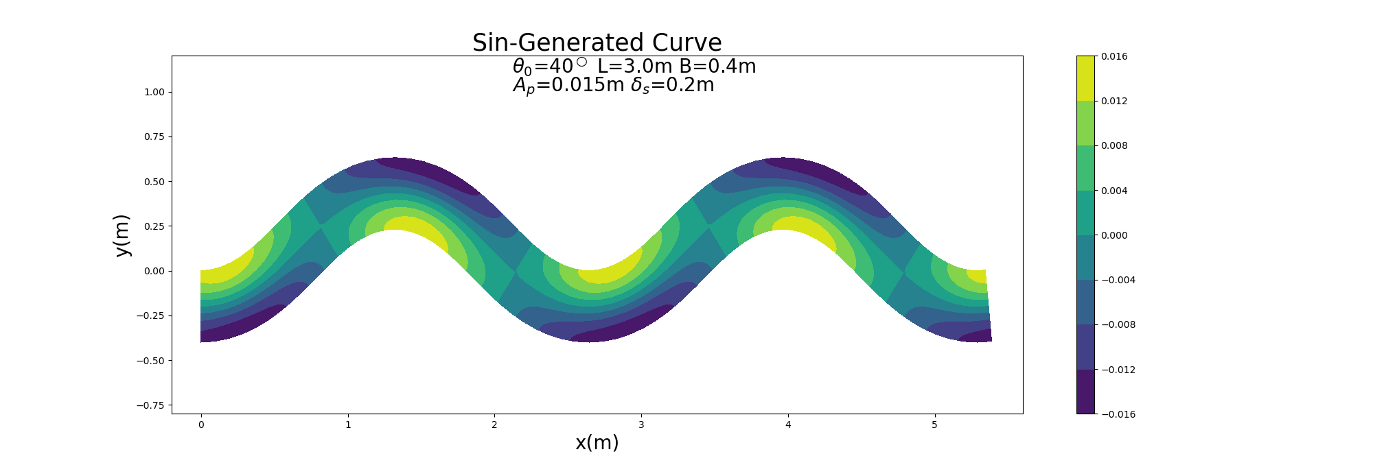
Figure 11.6 : The sine-generated curve channel used for calculation

The flow calculation is conducted for a flow with a discharge \(Q\) of 0.001 m \(^3\)/s flowing in this channel. Where, we assume a Manning’s coefficient of roughness \(n_m\) of 0.012 and a number of calculation grids of 41 \(\times\) grids per wavelength in the downstream direction. Therefore, we have 82 grids per two wavelengths and 21 grids in the transverse direction.

The calculation results are shown below. In this example, a sandbar-like bed is placed in the meander channel, with waterless floating bars alternating on the left and right. The current trial version of the code is not always accurate in handling the shoreline, resulting in flow instability near the shoreline. This is an area for further improvements, and you are welcome to share your ideas for improving the code.

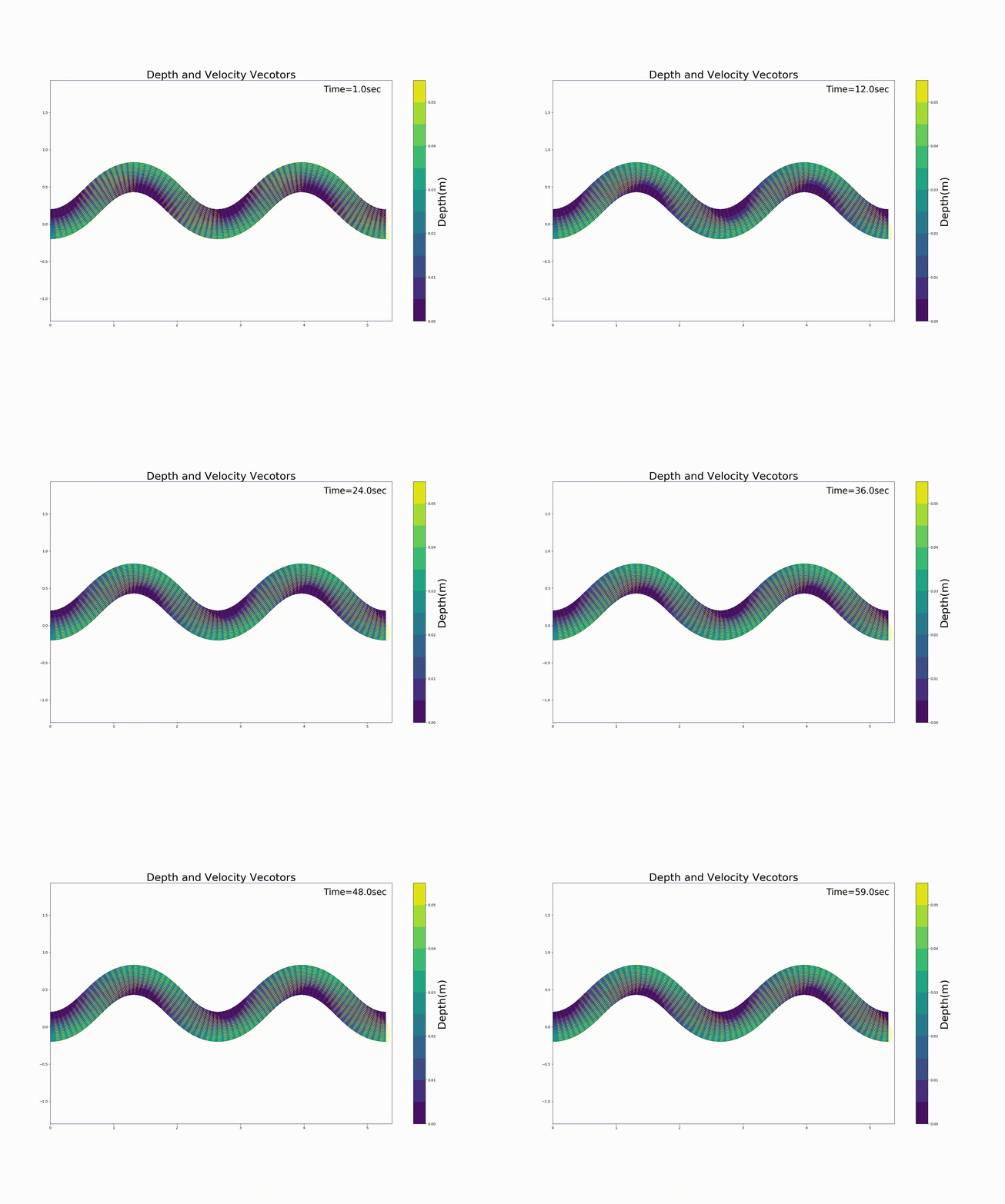
Figure 11.7 : Flow calculation results for a sine-generated curve channel (flow velocity vector and water depth)

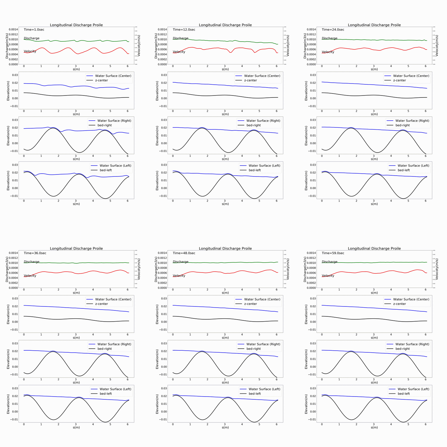
Figure 11.8 : Flow calculation results for a sine-generated curve channel (discharge and longitudinal profile of water level)

11.6. Periodic boundary conditions

Normally, for subcritical flow calculations, the discharge (velocity) is given for the upstreamend and the water level (water depth) is given for the downstreamend as the boundary conditions. In the calculations of Figure 11.7 and Figure 11.8, a constant discharge is given for the upstreamend and a constant water level is given for the downstreamend (in this case, the level of uniform flow). The Figure 11.9 shows how these boundary conditions are given in relation to the calculation points.

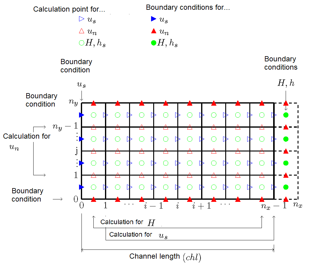
Figure 11.9 : Calculation grids and boundary conditions (for ordinary calculations)

In contrast, a method for giving the boundary conditions for an infinitely continuous channel, such as a meandering channel with sine-generated curves, is called the periodic boundary condition method. Using this method, the hydraulic quantities at the upstream and downstream ends are kept the same, enabling calculations that assume an endless channel.

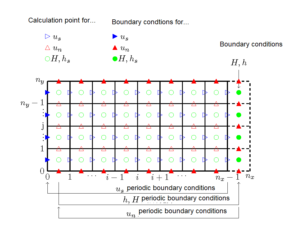
Figure 11.10 : Calculation grids and boundary conditions (for ordinary calculations)

For your reference, the code at https://github.com/YasuShimizu/Nays2d_sn_python

can address periodic boundary conditions. The calculation conditions are described in the “config.yml” file below. config.yml file (https://github.com/YasuShimizu/Nays2d_sn_python/blob/main/config.yml)

j_rep: 1 # the periodic boundary conditions (0: no periodic boundary conditions, 1: periodic boundary conditions)

By setting “1” for the parameter, j_rep, in the first line of the “config.yml file”, we can express the periodic boundary conditions. Figure 11.11 and Figure 11.12 are given by changing the calculation results of :numref:`sg_animation and Figure 11.8, which immediately precede, to the periodic boundary conditions. At first glance they look the same as the case without the periodic boundary conditions, but in fact the conditions are applied for this.

Figure 11.11 : Flow calculation results for a sine-generated curve channel (flow velocity vector and water depth) [periodic boundary conditions]

Figure 11.12 : Flow calculation results for a sine-generated curve channel (discharge and longitudinal profile of water level) [periodic boundary conditions]