10. Calculation of 2D flow in meandering channels(basic edition)

10.1. Sine-generated curve

10.1.1. Generating a sine-generated curve

According to Langbein and Leopold [Ref:33], the channel shape of a meandering river can be approximated by the following sine-generated curve. “Sine-generated curve” does not mean a curve whose planar coordinates on the river follow a sine curve; the “sine” refers to the sine function that is used to express the angle of the channel direction.

(10.1)\[\theta = \theta_0 \sin \cfrac{2\pi s}{L}\]

Where, \(s\) is the coordinate axis along the channel centerline, \(\theta\) is an angle from the horizontal direction of the \(s\) axis (the meandering deflection angle), \(\theta_0\) is the maximum meandering deflection angle, and \(L\) is the meandering wavelength (the length along the \(s\) axis). Figure 8.26, Figure 8.27 and Figure 8.28 are the simulation results using the sine-generated curves.

When using Equation (10.1) to draw a channel shape and when using that shape to perform analyses, such shape needs to be converted to \(x-y\) coordinates.

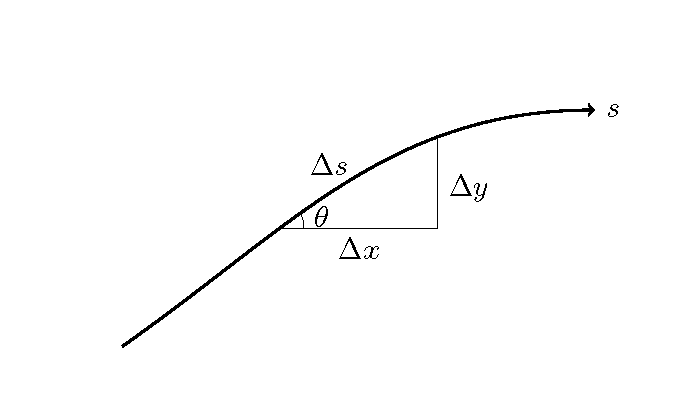
Figure 10.1 : Relationships between \(\Delta x, \Delta y, \Delta s\)

The components in the \(x,y\) directions of the infinitesimal element, \(\Delta s\), along the \(s\) axis are defined by Figure 10.1 as follows.

(10.2)\[\Delta x = \Delta s \cos\theta, \hspace{2cm} \Delta y = \Delta s \sin\theta\]

Then, \(s,x,y\) are given as follows.

(10.3)\[s=s_0 +\int_{s_0}^s ds, \hspace{1cm} x=x_0 +\int_{s_0}^s \cos\theta ds, \hspace{1cm} y=y_0 +\int_{s_0}^s \sin\theta ds\]

The actual calculation procedure is as follows.

1. Successively add infinitesimal \(\Delta s\) along the \(s\) axes.

2. At each addition, using Equation (10.1), obtain \(\theta\).

3. Using \(\theta\) and \(\Delta s\) defined above, obtain \(\Delta x\) and \(\Delta y\) with Equation (10.2).

4. By cumulating this, successively obtain the values of \(x, y\).

The Python code for this is as follows. https://github.com/YasuShimizu/Python-Code/blob/main/sg_plot.py

The code above plots four types of alignment for sine-generated curves when \(\theta_0\) are \(30^\circ, 60^\circ, 90^\circ, 120^\circ\). The wavelength, the wave number, and the like are specified in the code. The following figure shows the execution results of the code.

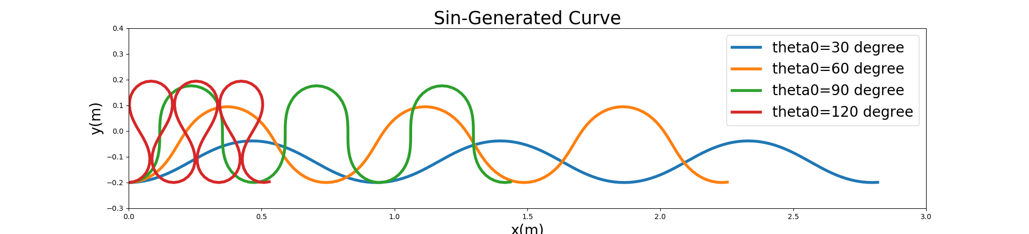
Figure 10.2 : Example of a sine-generated curve

10.1.2. Making calculation grids by using a sine-generated curve

The shapes shown by Figure 10.2 are the shapes of the centerline. When performing the 2D analysis, we need the coordinates of the right and left banks, and we need the coordinates of each grid obtained by dividing the right and left bank coordinates by the number of grids in the cross-sectional direction.

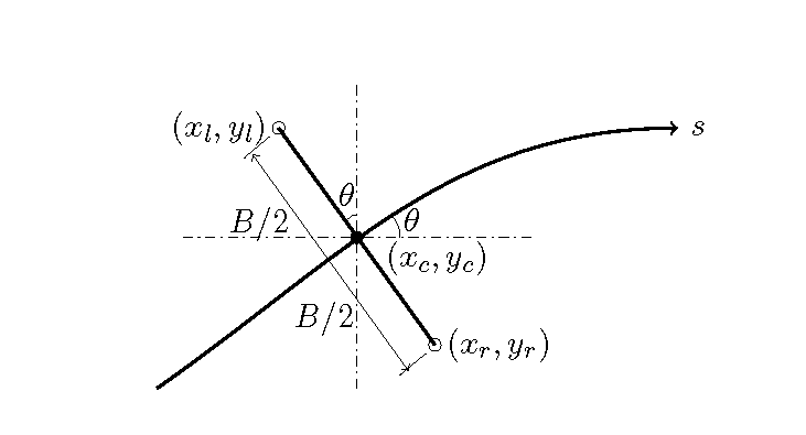
Figure 10.3 : Definitions of the right and left banks in a sine-generated curve

As shown by Figure 10.3, the coordinates of the right and left banks are the two points at a distance that is half the river width from the intersection between the \(s\) axis (the channel centerline) and a traversal line perpendicular to the axis. Assuming that the coordinates of the center of the channel and the grid points of the right and left banks are \((x_c, y_c), (x_r, y_r), (x_l, y_l)\), respectively, then the following equations are satisfied.

(10.4)\[ \begin{align}\begin{aligned}x_r=x_c+\cfrac{B}{2}\sin\theta, \hspace{2cm} & y_r=y_c-\cfrac{B}{2}\cos\theta\\x_l=x_c-\cfrac{B}{2}\sin\theta, \hspace{2cm} & y_l=y_c+\cfrac{B}{2}\cos\theta\end{aligned}\end{align} \]

Calculation grids are obtained by dividing the coordinates of the right and left banks with the given grid number.

The following is an example for \(\theta_0=40^\circ\).

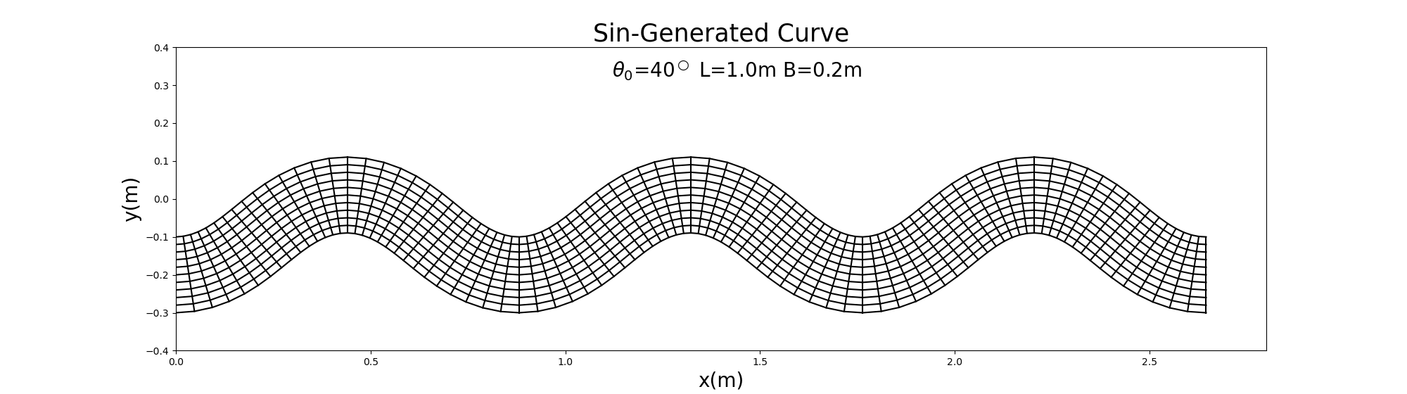
Figure 10.4 : Example of the calculation grids for the sine-generated curve when \(\theta=40^\circ\)

The Python code for generating this grid is as follows.

https://github.com/YasuShimizu/Python-Code/blob/main/sg_mkgrid40.py

For your reference, an example when \(\theta_0=100^\circ\) is below.

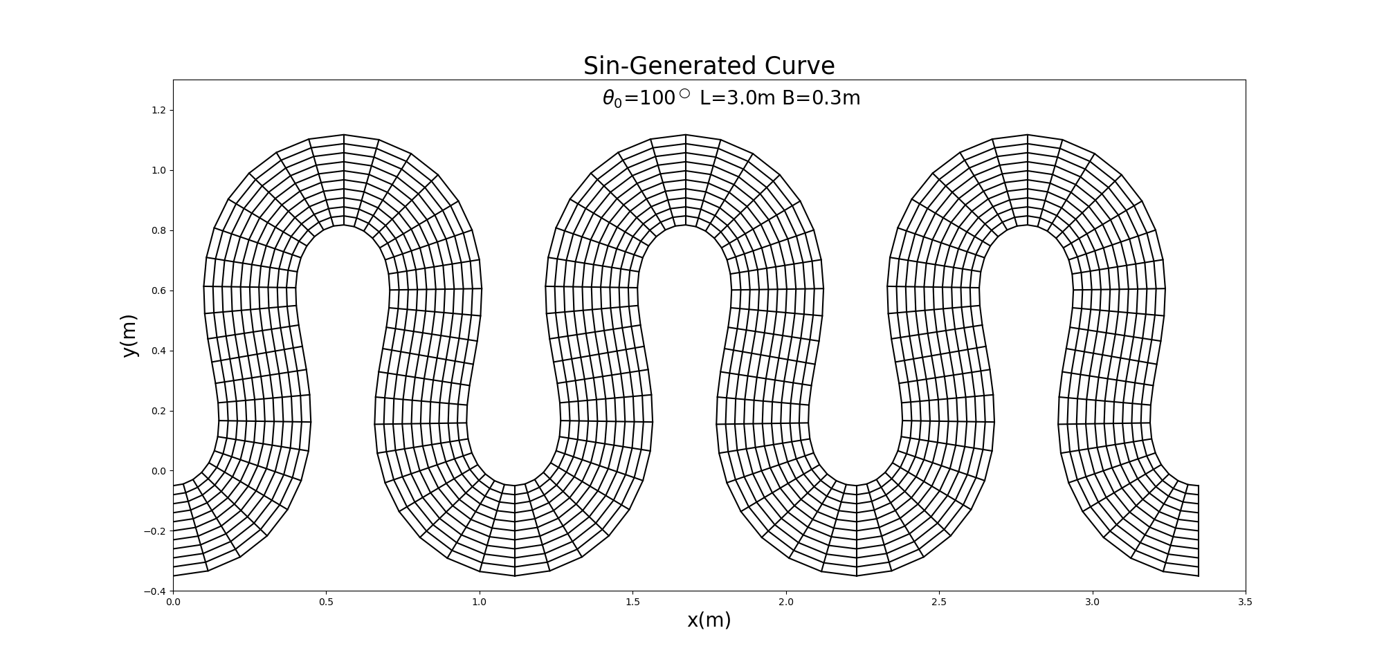
Figure 10.5 : Example of the calculation grids for the sine-generated curve when \(\theta=100^\circ\)

The Python code is below:

https://github.com/YasuShimizu/Python-Code/blob/main/sg_mkgrid100.py

10.1.3. Giving a “bar and pool” geometry to the bed

For the plane shape of the generated calculation grids Figure 10.5, the following equation can give sandbar-like relative heights on the bed.

(10.5)\[\Delta_z = -A_p\cos\left\{\cfrac{2\pi}{L}(s-\delta_s)\right\} \cos\left\{\cfrac{\pi}{B}n\right\}\]

Where, \(\Delta_z\) is the height relative to that of the bed, \(A_p\) is the sandbar wave-height, \(s\) is the distance along the channel centerline from the upstream end, \(n\) is the distance from the right bank to the left bank, and \(\delta s\) is the phase difference between the sandbar and the channel shape.

Using Equation (10.5), sandbar relative heights are arranged on a channel with a sine-generated curve as follows. Note that in this example, \(\theta_0=100^\circ\), \(L=\) 3.0 m, \(B=\) 0.3 m, \(A_p=\) 0.03 m, and \(\delta_s=\) 0.1 m.

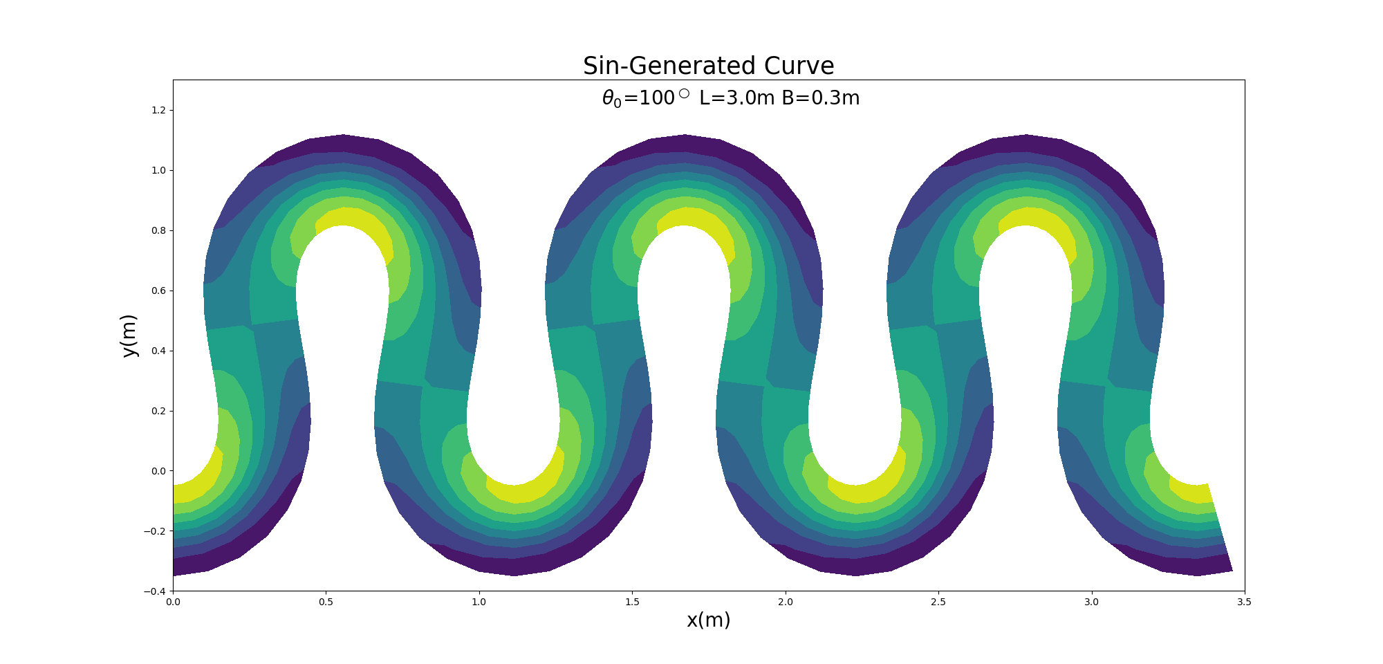
Figure 10.6 : Example of a rendering of a sandbar-like bed on the sine-generated curve when \(\theta=100^\circ\)

The Python code for calculating and rendering Figure 10.6 is as follows.

https://github.com/YasuShimizu/Python-Code/blob/main/sg_mkgrid_dz.py

10.2. Kinoshita meandering curve (meander curve proposed by Kinoshita)

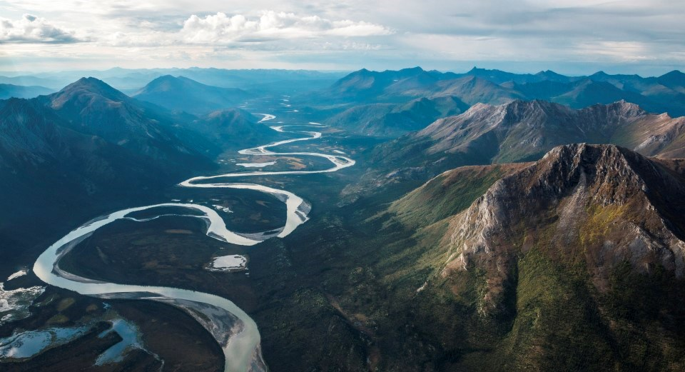
According to Abad and Garcia [Ref:34], by adding an additional term to Equation (10.1), such as that shown below, it is possible to reproduce the meandering shape of a natural river, such as Figure 10.7.

(10.6)\[\theta = \theta_0 \sin \cfrac{2\pi s}{L} +{\theta_0}^3\left\{J_s \cos\left(3\cfrac{2\pi s}{L}\right) -J_f \sin\left(3\cfrac{2\pi s}{L}\right) \right\}\]

Where, \(J_s\) and \(J_n\) are factors that show skewness and flatness, respectively.

Figure 10.7 : The Alatna River in Alaska, U.S.A. [Ref:35]

In Equation (10.6), assuming that \(\theta_0=100^\circ\), \(L\) =2.8m, \(B\) =0.2m, and \(J_s=1/32, J_f=1/192\), channel calculation girds are generated and shown in Figure 10.8. Abad and Garcia [Ref:34] call this channel planar shape the Kinoshita-generated meander curve, after the tortuous meander of Kinoshita [Ref:24].

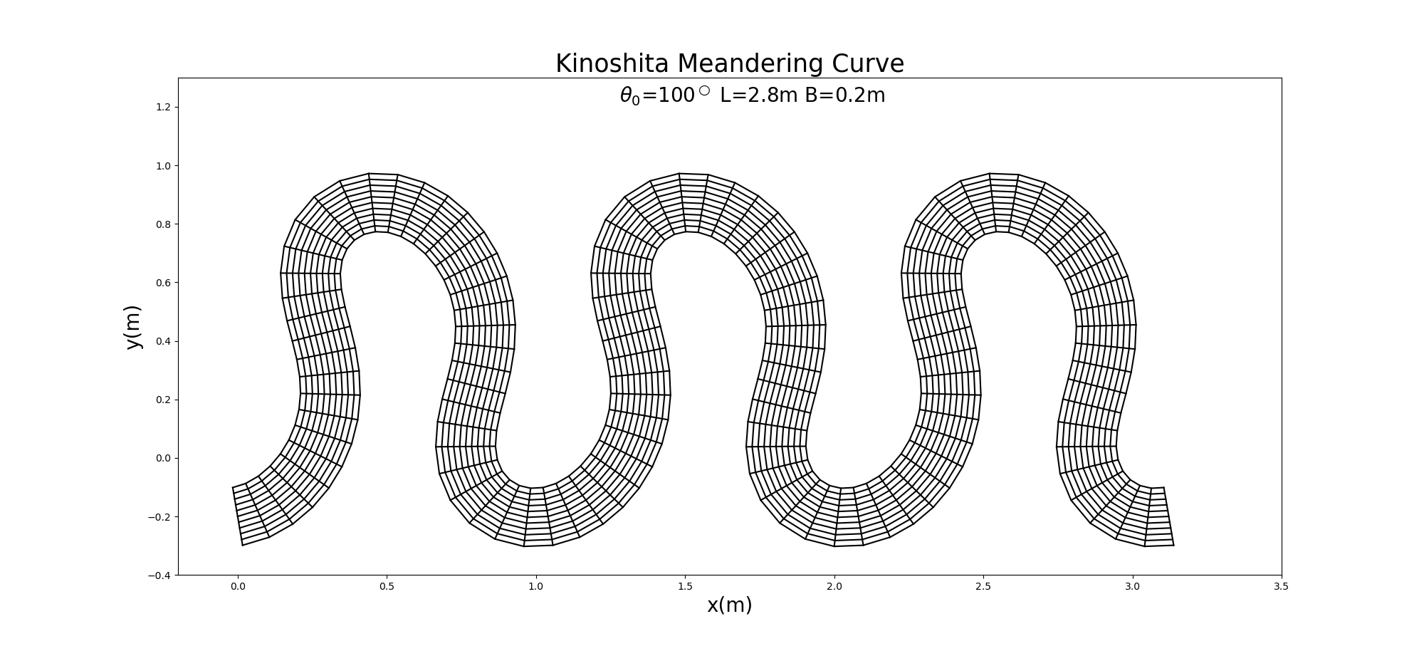
Figure 10.8 : A Kinoshita meander curve channel

The Python code for generating calculation grids for Figure 10.8 is as follows.

https://github.com/YasuShimizu/Python-Code/blob/main/kinoshita100.py

The Kinoshita-generated meander curve in Figure 10.8 can reproduce a bed topography that models the sandbar geometry of an actual river by giving the relative height on the sandbar in Equation (10.6).

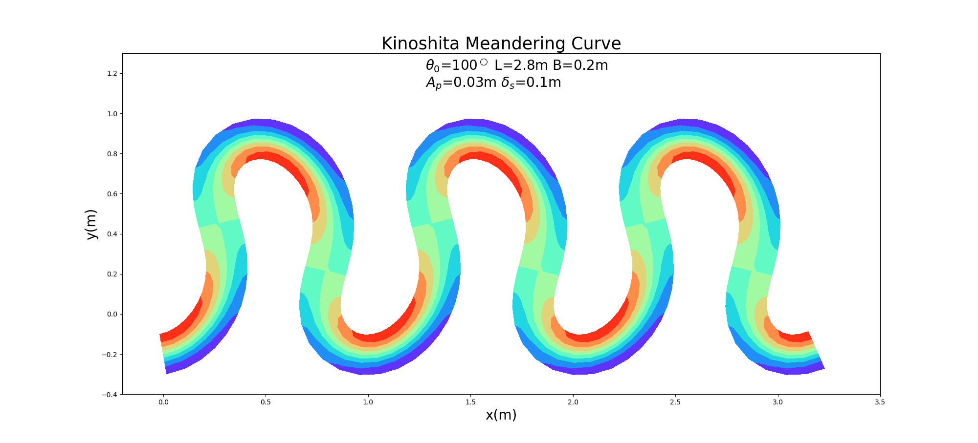
Figure 10.9 : Pool and bar geometry bed on the Kinoshita-generated curve when \(\theta=100^\circ\), \(A_p=\) 0.03m, and \(\delta_s=\) 0.1m.

The Python code for rending Figure 10.9 is below.

https://github.com/YasuShimizu/Python-Code/blob/main/kinoshita100_dz.py

10.3. Calculation of the sinuosity

For the above sine-generated curve and the Kinoshita-generated curve, the sinuosity of the channel is given by…

(10.7)\[\cfrac{1}{r}= \cfrac{\partial \theta}{\partial s}\]

For example, for the sine-generated curve in Equation (10.1), the sinuosity is given as follows.

(10.8)\[\cfrac{1}{r}=\cfrac{\partial \theta}{\partial s} = \cfrac{2\pi}{L}\theta_0 \cos \cfrac{2\pi n}{L}\]

However, the shape of a river tends not to conform exactly to the functional form described above. The sinuosity is calculated from various arbitrary shapes, both for natural and artificial channels.

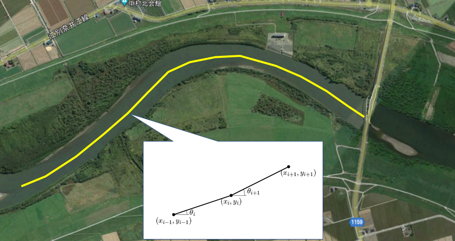
Figure 10.10 : Calculating the radius of curvature from the planar coordinates

As shown in Figure 10.10 , when there are planar coordinates along the center of the channel, the radius of curvature can be obtained by using Equation (10.7) in a discrete manner. Now,

(10.9)\[\cfrac{d}{ds}\left(\cfrac{dy}{dx}\right)=\cfrac{d}{ds}\tan\theta =\cfrac{1}{\cos^2\theta}\cfrac{d\theta}{ds}\]

Therefore,

(10.10)\[\cfrac{1}{r}=\cos^2\theta\cfrac{d}{ds} \left(\cfrac{dy}{dx}\right)\]

Using the symbols shown in Figure 10.10, we define the following.

(10.11)\[\begin{split}\Delta x_i=x_i-x_{i-1}, \hspace{1cm} \Delta y_i=y_i-y_{i-1}, \hspace{1cm} \Delta s_i =\sqrt{\Delta x_x^2 + \Delta y_i^2} \\ \cos\theta_i = \cfrac{\Delta x_i}{\Delta s_i}, \hspace{4cm} \sin\theta_i = \cfrac{\Delta y_i}{\Delta s_i} \hspace{3cm}\end{split}\]

Then, we have…

(10.12)\[ \begin{align}\begin{aligned}\cfrac{1}{r}=\cos^2\theta \cfrac{d}{ds}\left(\cfrac{dy}{dx}\right) =\cfrac{\Delta x^2}{\Delta s^2} \cfrac{\Delta x \cfrac{d(\Delta y)}{ds}-\Delta y \cfrac{d(\Delta x)}{ds}}{\Delta x^2}\\=\cfrac{1}{{\Delta s_i}^2} \left[ \Delta x \left\{ \sin\theta_{i+1}-\sin\theta_i \right\} -\Delta y \left\{ \cos\theta_{i+1} - \cos\theta_i \right\} \right]\\=\cfrac{1}{\Delta s_i} \left[ \cos\theta_i \left\{\sin\theta_{i+1}-\sin\theta_i \right\} -\sin\theta_i \left\{ \cos\theta_{i+1} - \cos\theta_i \right\} \right]\end{aligned}\end{align} \]

The results of comparison between the analytically calculated curvature that is obtained by applying (10.8) to the sine-generated curve and the numerically calculated curvature that is obtained by using Equation (10.12) are shown in the figure below. The blue line represents analytical solutions, and the orange line represents numerical solutions. This is an example where the meander deviation angle is \(\theta_0=90^\circ\). As you can see, the analytical and numerical solutions almost perfectly correspond to each other.

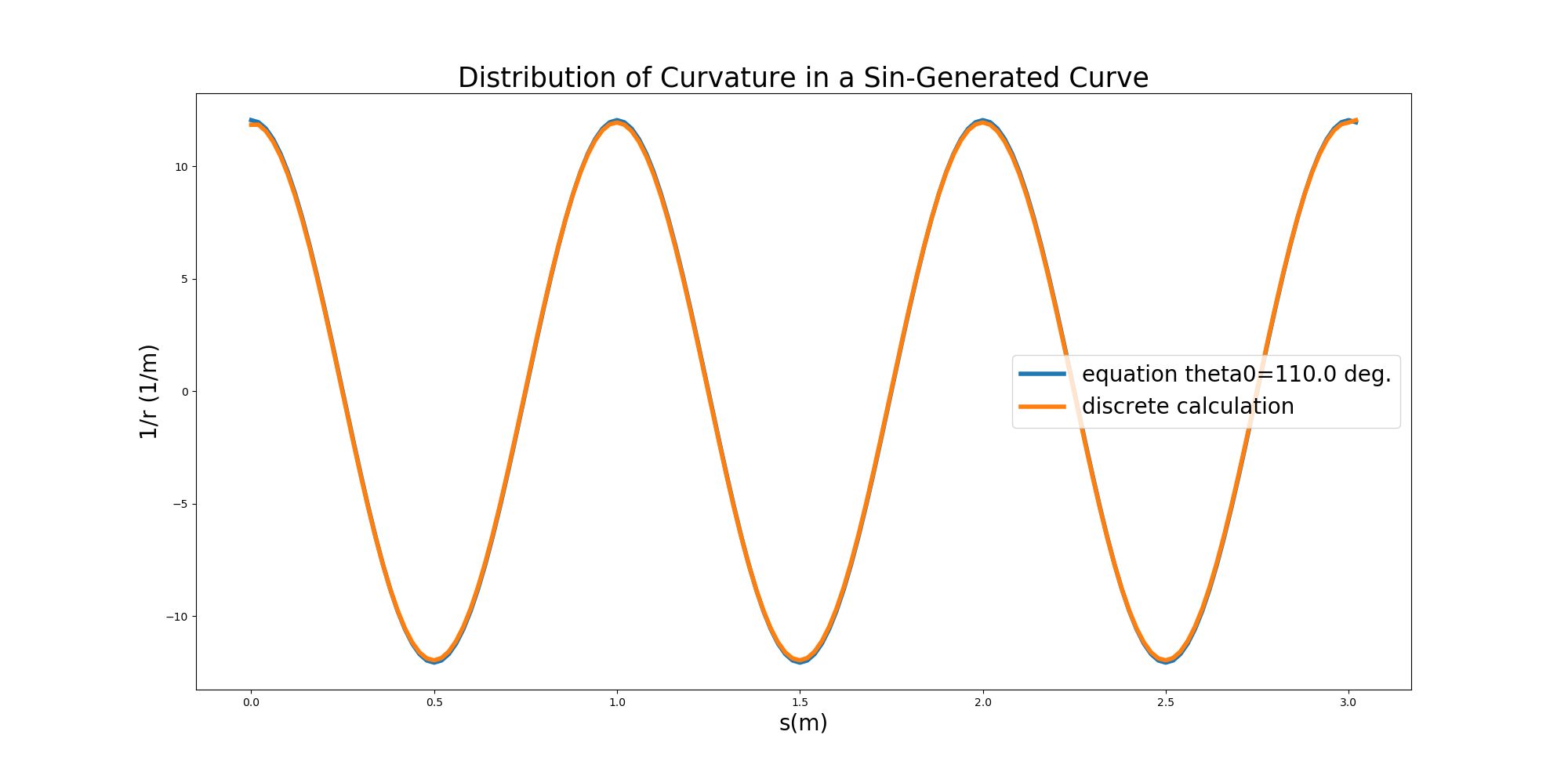
Figure 10.11 : Verification example for a curvature calculation method using numerical calculation

The Python code for calculating and rendering Figure 10.11 are as follows.

https://github.com/YasuShimizu/Python-Code/blob/main/radius_cmp.py