Appendix III (Diffusion equation in the s-n coordinates)

Derivation of the diffusion equation in the s-n coordinates

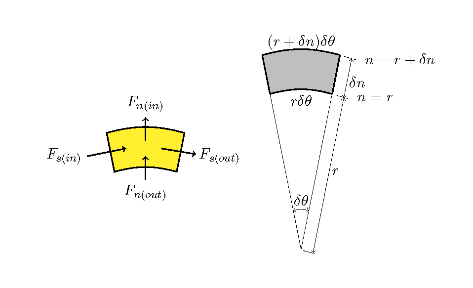
Let us assume that the \(s-n\) coordinates are Cartesian curvilinear coordinates. On the \(s-n\) coordinates, the \(s\) axis is assumed to be an arbitrary curve, and the \(n\) axis is assumed to be a straight coordinate axis perpendicular to the s axis.

Figure 12 : Density flux balance of the infinitesimal elements on the \(s-n\) coordinates

Assuming that the density of the diffusion material is \(c\), then the unit width flux and the diffusion coefficient in the \(s, n\) direction are \(F_s, F_n\) and \(D_s, D_n\), respectively. They have following relationships.

(114)\[F_s=-D_s\cfrac{\partial F_s}{\partial s}, \hspace{2cm} F_n=-D_n\cfrac{\partial F_n}{\partial n}\]

Considering the density balance of the infinitesimal elements in an infinitesimal time shown in Figure 12 and taking into account that the area of the infinitesimal element is \(r\, \delta\theta\, \delta n\), then, the following equations are derived.

(115)\[\cfrac{\partial c}{\partial t} r\, \delta\theta\, \delta n =F_{n(n)}r \delta\theta - F_{n(n+\delta n)} (r+\delta n) \delta\theta +F_{s(s)}\delta n -F_{s(s+\delta s)}\delta n\]

(116)\[\cfrac{\partial c}{\partial t}=\cfrac{F_{n(n)}}{\delta n}-\cfrac{F_{n(n+\delta n)}\, (r+\delta n)}{r\delta n} +\cfrac{F_{s(s)}-F_{s(s+\delta s)}}{\delta s}\]

Where,

(117)\[\cfrac{(r+\delta n)}{r\delta n}=\cfrac{1}{r}+\cfrac{1}{\delta n}\]

Therefore, the second term on the right side of Equation (116) is…

(118)\[\cfrac{F_{n(n+\delta n)}\, (r+\delta n)}{r\delta n}= \cfrac{F_{n(n+\delta n)}}{r}+\cfrac{F_{n(r+\delta n)}}{\delta n}\]

Then, Equation (116) is expressed as follows.

(119)\[ \begin{align}\begin{aligned}\cfrac{\partial c}{\partial t} & =\cfrac{F_{n(n)}}{\delta n}-\cfrac{F_{n(n+\delta n)}}{\delta n} -\cfrac{F_{n(n+\delta n)}}{r}+\cfrac{F_{s(s)}-F_{s(s+\delta s)}}{\delta s}\\& =-\cfrac{\partial F_n}{\partial n}-\cfrac{1}{r}F_{n(r+\delta n)}-\cfrac{\partial F_s}{\partial s}\\& =\cfrac{\partial}{\partial s}\left(D_s \cfrac{\partial c}{\partial s}\right) +\cfrac{\partial}{\partial n}\left(D_n\cfrac{\partial c}{\partial n}\right) +\cfrac{D_n}{r}\cfrac{\partial c}{\partial n}\end{aligned}\end{align} \]

When \(D_s=D_n=D\),

(120)\[\cfrac{\partial c}{\partial t}=D \left( \cfrac{\partial^2 c}{\partial s^2}+\cfrac{\partial^2 c}{\partial n^2}+ \cfrac{1}{r}\cfrac{\partial c}{\partial n} \right)\]

Derivation of the equation of continuity on the s-n coordinates (alternative solution)

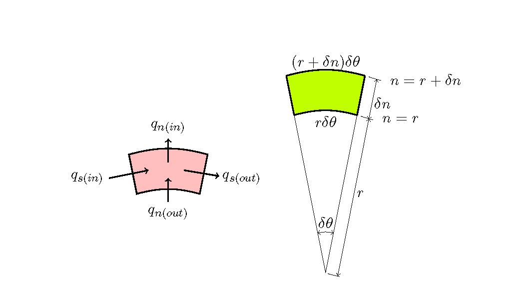
Let us assume that the \(s-n\) coordinates are Cartesian curvilinear coordinates. On the \(s-n\) coordinates, the \(s\) axis is assumed to be an arbitrary curve, and the \(n\) axis is assumed to be a straight coordinate axis perpendicular to the s axis.

Figure 13 : Flux balance of the infinitesimal elements on the \(s-n\) coordinates

\(q_s, q_n\) is the flow flux. Considering the flow flux balance of the infinitesimal elements in an infinitesimal time shown in Figure 13, and taking into account that the area of the infinitesimal element is \(r\, \delta\theta\, \delta n\), following equations are derived.

(121)\[\cfrac{\partial h}{\partial t} r\, \delta\theta\, \delta n =q_{n(n)}r \delta\theta - q_{n(n+\delta n)} (r+\delta n) \delta\theta +q_{s(s)}\delta n -q_{s(s+\delta s)}\delta n\]

(122)\[\cfrac{\partial h}{\partial t}=\cfrac{q_{n(n)}}{\delta n}-\cfrac{q_{n(n+\delta n)}\, (r+\delta n)}{r\delta n} +\cfrac{q_{s(s)}-q_{s(s+\delta s)}}{\delta s}\]

Where, \(h\) is the mean water depth for the infinitesimal elements. Then,

(123)\[\cfrac{(r+\delta n)}{r\delta n}=\cfrac{1}{r}+\cfrac{1}{\delta n}\]

Therefore, the second term of the right side of Equation (122) is…

(124)\[\cfrac{q_{n(n+\delta n)}\, (r+\delta n)}{r\delta n}= \cfrac{q_{n(n+\delta n)}}{r}+\cfrac{q_{n(r+\delta n)}}{\delta n}\]

Then, Equation (122) is expressed as follows.

(125)\[ \begin{align}\begin{aligned}\cfrac{\partial h}{\partial t} & =\cfrac{q_{n(n)}}{\delta n}-\cfrac{q_{n(n+\delta n)}}{\delta n} -\cfrac{q_{n(n+\delta n)}}{r}+\cfrac{q_{s(s)}-q_{s(s+\delta s)}}{\delta s}\\& =-\cfrac{\partial q_n}{\partial n}-\cfrac{1}{r}q_{n(r+\delta n)}-\cfrac{\partial q_s}{\partial s}\end{aligned}\end{align} \]

Where,

(126)\[\cfrac{\partial(rq_n)}{\partial n}=r\cfrac{\partial q_n}{\partial n}+q_n\cfrac{\partial r}{\partial n}=r\cfrac{\partial q_n}{\partial n}+q_n\]

Consequently,

(127)\[\cfrac{1}{r}\cfrac{\partial(rq_n)}{\partial n}=\cfrac{\partial q_n}{\partial n}+\cfrac{q_n}{r}\]

Therefore,

(128)\[\cfrac{\partial h}{\partial t}+\cfrac{\partial q_s}{\partial s}+\cfrac{1}{r}\cfrac{\partial(rq_n)}{\partial n}=0\]

or,

(129)\[\cfrac{\partial h}{\partial t}+\cfrac{\partial(hu_s)}{\partial s}+\cfrac{1}{r}\cfrac{\partial(rhu_n)}{\partial n}=0\]