9. One dimensional bed deformation modeling

9.1. With bedload sediment transport

9.1.1. Continuity equation for bedload sediment transport

The 1D equation of continuity for sediment transport in a channel with a rectangular cross-section is as follows.

(9.1)\[ \cfrac{\partial z_b}{\partial t}+\cfrac{1}{(1-\lambda)B} \cfrac{\partial(B q_b)}{\partial x}=0\]

Where, \(B\) is the channel width and \(\lambda\) is the void ratio of the riverbed materials.

The concept of Equation (9.1) is shown in Figure 9.1. As shown in the figure, as a result of the balance of sediment transport between two cross-sections separated by a distance of \(\Delta x\), the balance is assumed to continue for \(\Delta t\), and the riverbed elevation is assumed to change by \(\Delta z_b\). The reason for incorporating void ratio is that the bed deformation volume from deposition or erosion that results from the balance of sediment transport contains voids, \(\lambda\).

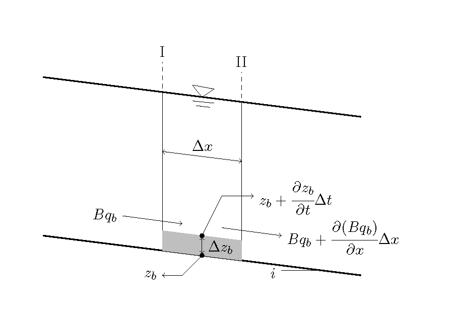
Figure 9.1 : Schematic of 1D riverbed deformation (bedload)

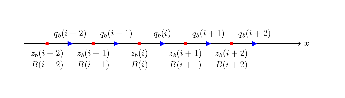
Figure 9.2 : Staggered grid (1D riverbed deformation calculation)

When the calculation grid for bedload is arranged as shown in Figure 9.2, the difference expression of Equation (9.1) is given by the following equation. Note that the calculation points for \(q_b\) are the same as those for \(u\) in Figure 5.1. And the calculation points for \(z_b\) are the same as those for \(h\) in Figure 5.1.

(9.2)\[z_b(i)^{n+1}=z_b(i)^n-\cfrac{\Delta t}{(1-\lambda)B(i)\Delta x} \left\{q_b(i)B_u(i)-q_b(i-1)B_u(i-1)\right\}\]

Where, \(B_u\) is the value of \(B\) at the calculation points of \(q_b\). The value of math: q_b(i) at each calculation point is given by Equation (8.22) and Equation (8.23). The values of \(\tau_\ast\) used for these sediment transport equations are given by Equation (8.10). Here, \(I_e\), which is used for Equation (8.10), is given by the following equation when the Manning formula is applied.

(9.3)\[I_e= \cfrac{{n_m}^2 u^2}{h^{4/3}}\]

9.1.2. Calculation procedure

The calculation procedure is shown by the following flowchart: The bed deformation calculated by Equation (9.2) is added to the end of Figure 5.3.

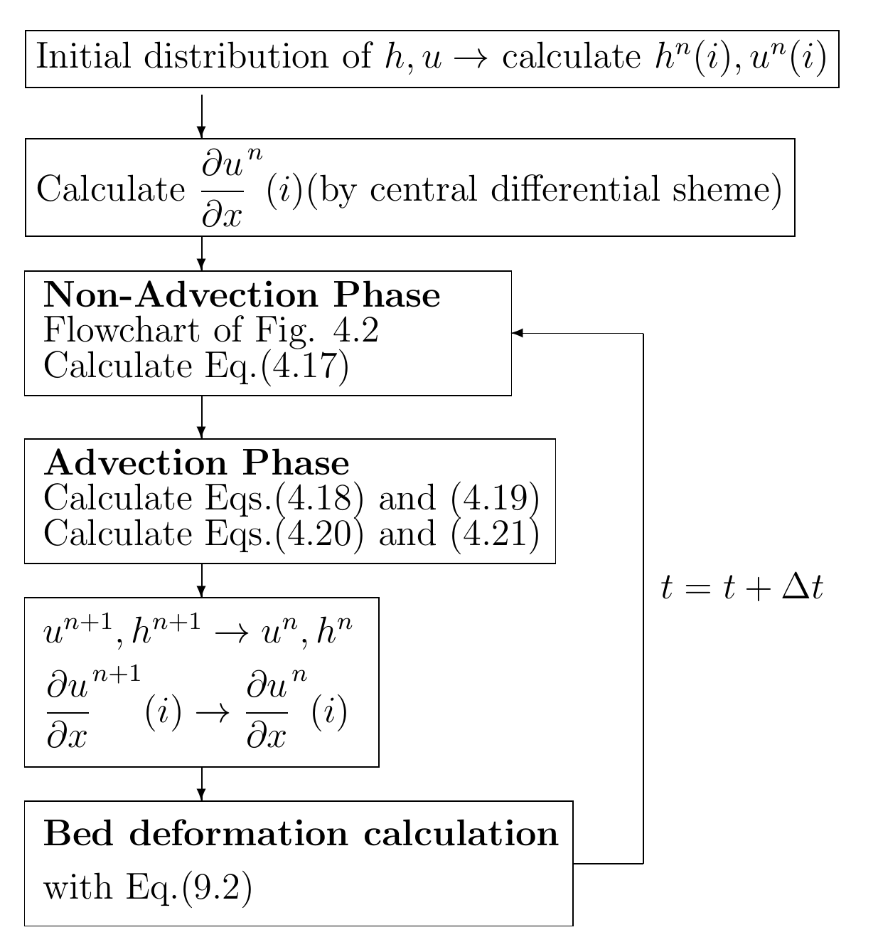
Figure 9.3 : Flowchart for 1D calculation of riverbed deformation

9.1.3. The Python code

The Python code for the above calculation procedure is given here.

https://github.com/YasuShimizu/1D_Flow_and_Bed_Deformation

The main body of the calculation code is in “main.py” of this repository, from which we can access the respective “function.py” files that have been listed in the repository. Calculation conditions are set with “yml” files in the repository. The following four files for calculation condition are included.

1. Bed deformation for a river with a mound near the longitudinal midpoint of the channel: config_mound.yml

2. Bed deformation for a river with a constraint near the longitudinal midpoint of the channel: config_constriction.yml

3. Bed deformation for a river with a gradient changing point: config_slope_change.yml

4. Bed deformation for a river with no bedload supply from upstream (a section below a dam): downstream_dam.yml

To execute these calculations, for example for “1.” above, in the prompt of Miniconda, write

> python main.py config_mound

for “xxxx” in “config_xxxxx.yml” which is a parameter as well as the file name. Then, to execute the calculation the yml file that describes the condition is called up.

9.1.4. Calculation results

The calculation results for 1D bed deformation under the above four conditions are as follows.

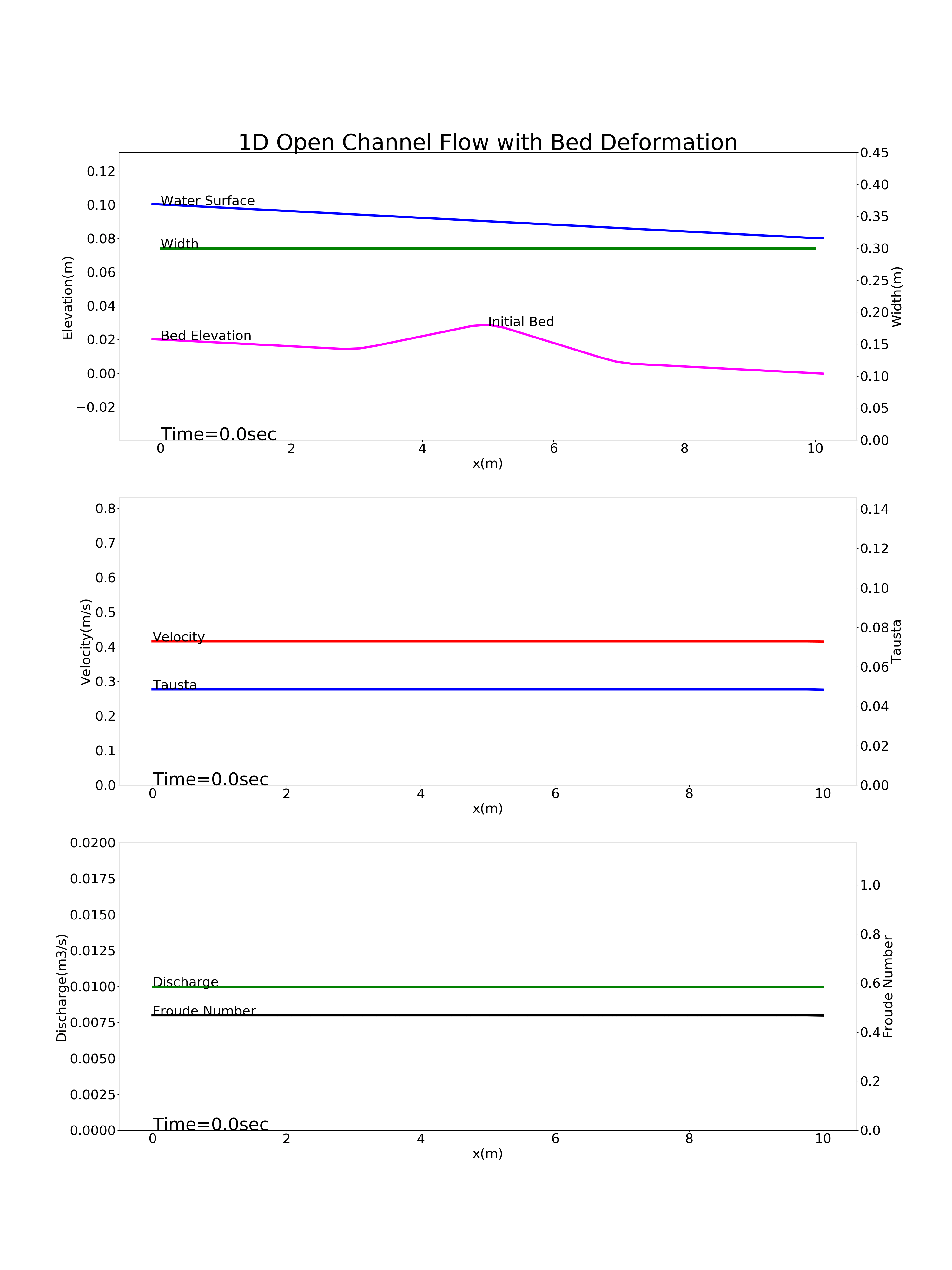
Figure 9.4 : Calculation results for the bed deformation of a river with a mound near the longitudinal midpoint of the channel

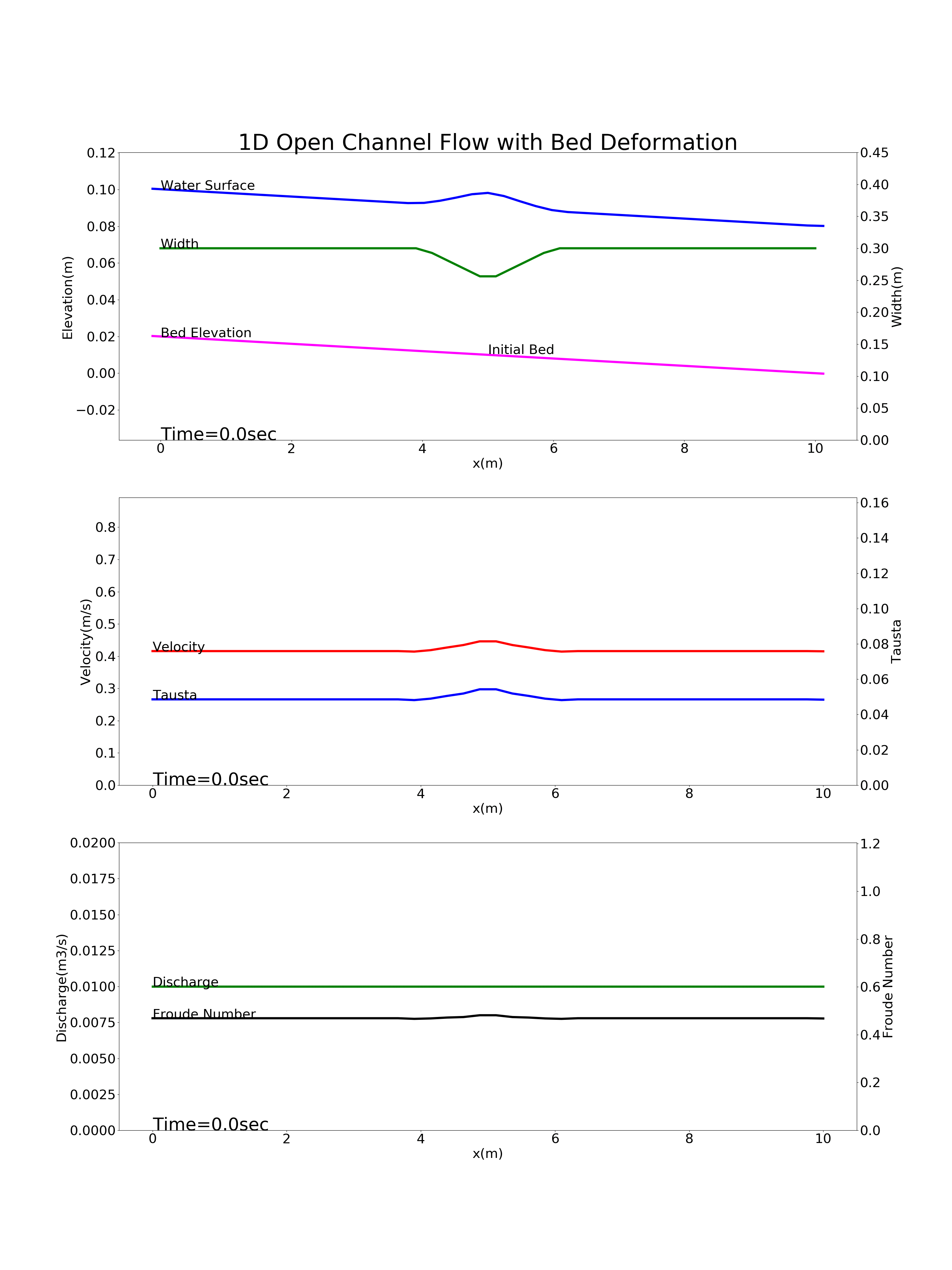
Figure 9.5 : Calculation results for the bed deformation of a river with a constraint near the longitudinal midpoint of the channel

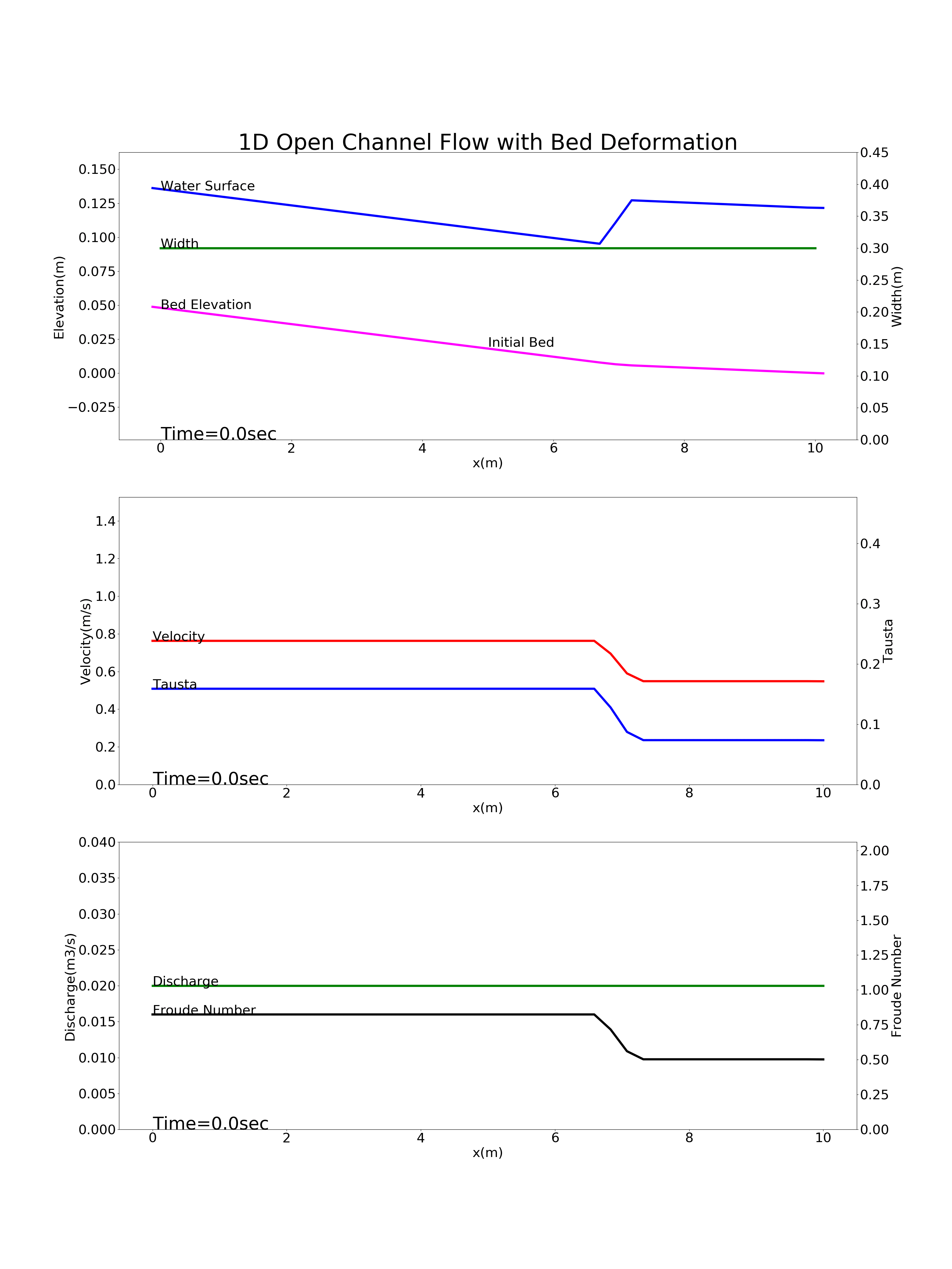
Figure 9.6 : Calculation results for the bed deformation of a river with a gradient changing point

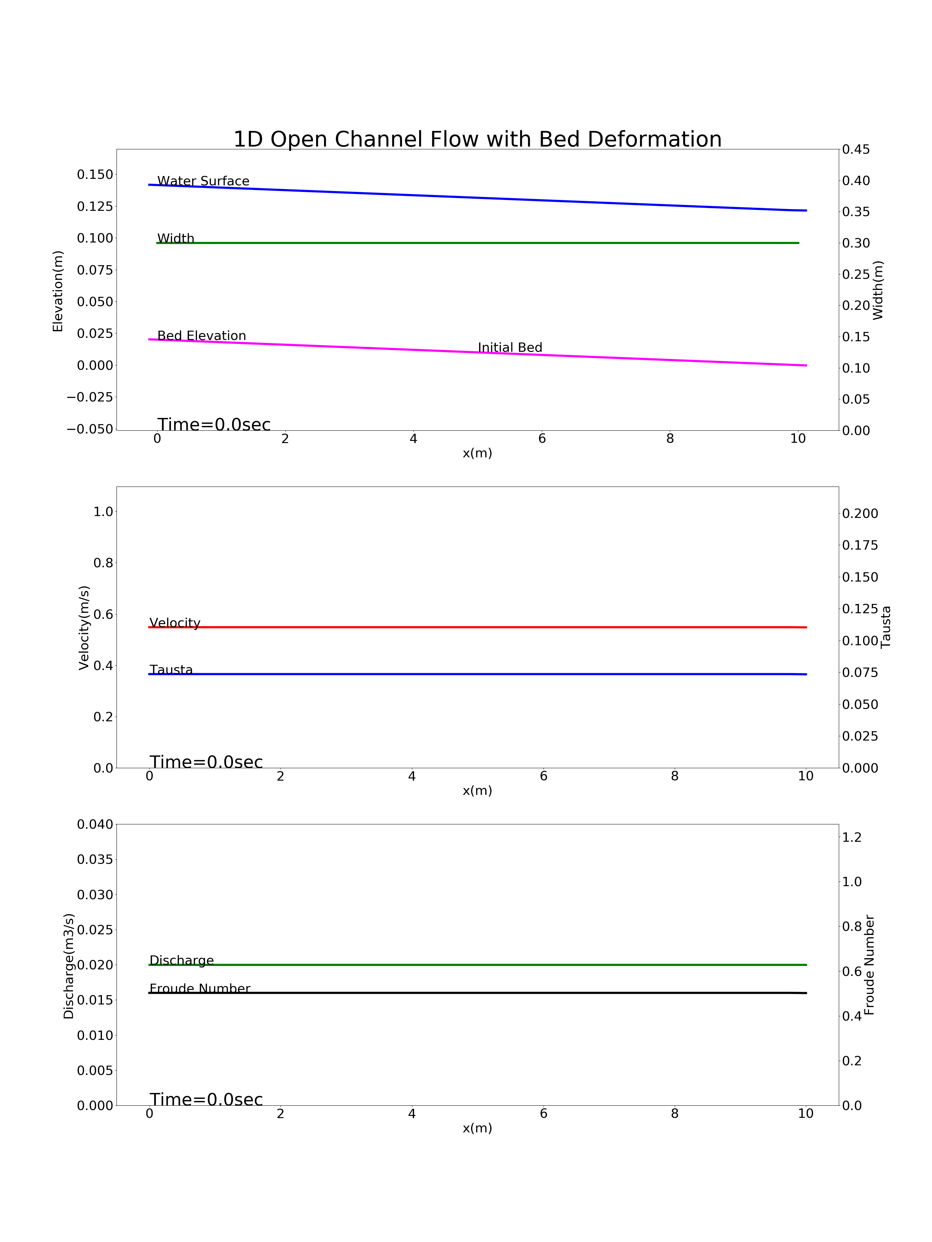
Figure 9.7 : Calculation results for the bed deformation of a river with no bedload supply from upstream (a section immediately downstream of a dam)

9.2. With suspended load sediment transport

9.2.1. Continuity equation for suspended sediment concentration

As shown in Figure 9.8, we assume a channel with a rectangular cross-section and two cross-sections (I and II) that are separated by a distance of \(\Delta x\), to consider the continuous conditions of suspended sediment.

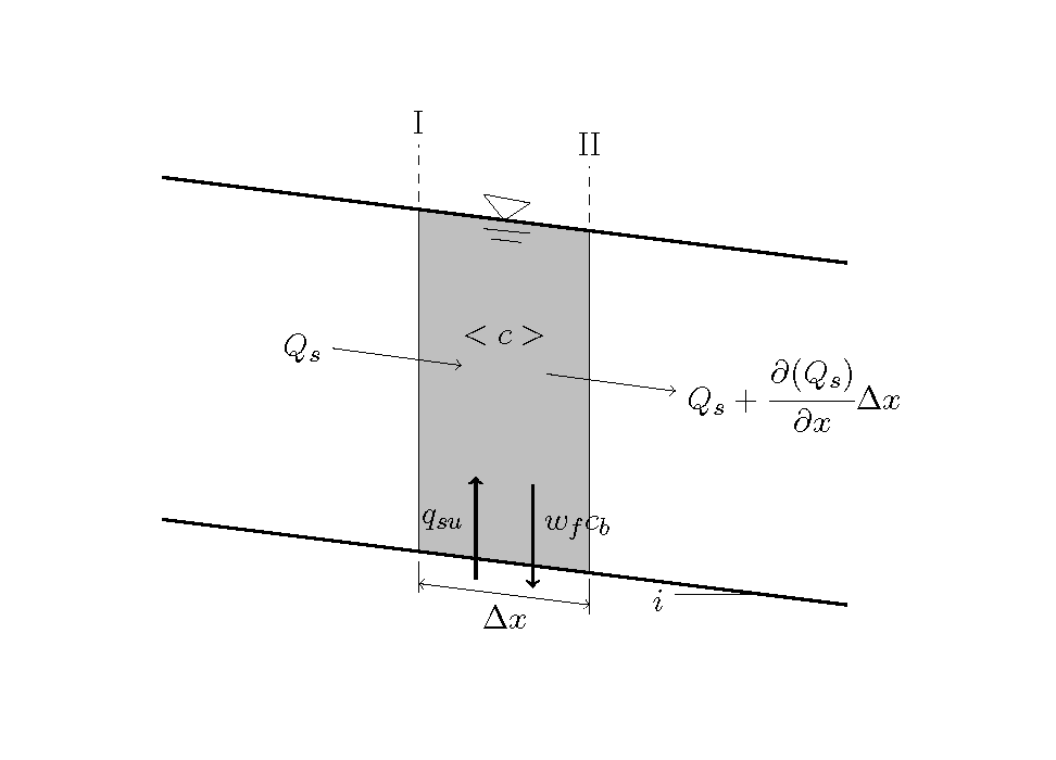
Figure 9.8 : Conceptual diagram for continuous conditions of the 1D suspended sediment

In the above \(\Delta x\) section, assuming that the volume of water is \(V\), the average concentration is \(<c>\), the average water depth is \(h\), the average channel width within the section is \(B\), and the amount of suspended sediment transported through the section is \(Q_s\), then we have…

(9.4)\[\cfrac{\partial(V<c>)}{\partial t} \Delta t + \cfrac{\partial{Q_s}}{\partial x} \Delta x \Delta t =(q_{su}-w_f c_b) \Delta x \Delta t B\]

Where, \(q_{su}\) is the amount of suspended sediment supplied from the bed per unit area per unit time, \(w_f\) is the sediment settling velocity, and \(c_b\) is the suspended sediment concentration near the bed. Also, because

(9.5)\[V=A\Delta x = BH \Delta x, \; \; \; Q_s=Q<c>=Bhu<c>\]

Therefore,

(9.6)\[\begin{split}\cfrac{\partial(V<c>)}{\partial t}=B \Delta x \cfrac{\partial}{\partial t} (h<c>) \\ \cfrac{\partial Q_S}{\partial x}=\cfrac{\partial}{\partial x}(Bhu<c>)\end{split}\]

Therefore, Equation (9.4) is…

(9.7)\[\cfrac{\partial(h<c>)}{\partial t} B \cancel{\Delta x \Delta t} + \cfrac{\partial(Bhu<c>)}{\partial x} \cancel{\Delta x \Delta t} = (q_{su}-w_f c_b) B \cancel{\Delta x \Delta t}\]

In addition…

(9.8)\[<c>\cfrac{\partial h}{\partial t}+ h\cfrac{\partial<c>}{\partial t}+ \cfrac{1}{B} \left\{ <c>\cfrac{\partial(Bhu)}{\partial x}+ Bhu\cfrac{\partial<c>}{\partial x} \right\} =q_{su}-w_f c_b\]

(9.9)\[<c> \cancelto{\mbox{ from the equation of continuity }=0}{\left\{ \cfrac{\partial h}{\partial t} + \cfrac{1}{B} \cfrac{\partial(Buh)}{\partial x} \right\}} + h\cfrac{\partial<c>}{\partial t} + hu \cfrac{\partial<c>}{\partial x} =q_{su}-w_f c_b\]

Therefore,

(9.10)\[\cfrac{\partial<c>}{\partial t} + u \cfrac{\partial<c>}{\partial x} =\cfrac{1}{h}(q_{su}-w_f c_b)\]

By applying the relationship given by Equation (8.38) for \(<c>\) and \(c_b\) in Equation (9.10), we have…

(9.11)\[\cfrac{\partial<c>}{\partial t} + u \cfrac{\partial<c>}{\partial x} =\cfrac{1}{h}(q_{su}-\alpha w_f <c>)\]

Where,

(9.12)\[\alpha=\cfrac{\beta}{1-\exp(-\beta)}, \; \; \beta=\cfrac{w_f h}{\epsilon}\]

When incorporating diffusion of the suspended sediment concentration, add a diffusion term to the right side of (9.11). Then, we have the following equation.

(9.13)\[\cfrac{\partial<c>}{\partial t} + u \cfrac{\partial<c>}{\partial x} = D\cfrac{\partial ^2<c>}{\partial x^2}+ \cfrac{1}{h}(q_{su}-\alpha w_f <c>)\]

Consequently, Equation (9.13) is the equation of continuity for the depth-averaged suspended sediment concentration. The difference method is used for calculation of the equation. Equation (9.13) has the same form as Equation (3.29) which is an advection equation with a source term. It is given by replacing \(f\) with \(<c>\) and \(G\) with \(D\cfrac{\partial ^2<c>}{\partial x^2}+\cfrac{1}{h}(q_{su}-\alpha w_f <c>)\) in Equation (3.29). \(D\cfrac{\partial ^2<c>}{\partial x^2}+\cfrac{1}{h}(q_{su}-\alpha w_f <c>)\) Use of the CIP method, which has been applied in this text, realizes highly accurate calculations. Also, in the calculation of \(<c>\), the calculation point is arranged between the calculation points of \(u\), as shown in the following figure. Therefore, the calculation point (9.14) is newly defined as \(u\) at the calculation point of \(<c>\), as shown in Equation \(u_x\). This (9.14) is used as the advection velocity, \(u\), in the calculation of Equation (9.11).

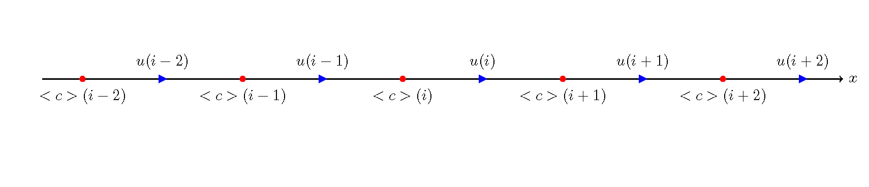
Figure 9.9 : Arrangement of calculation points for suspended sediment concentration

(9.14)\[u_x(i)=\cfrac{u(i)+u(i-1)}{2}\]

9.2.2. Continuity equation for the bed with suspended sediment transport

The suspended sediment concentration close to the bed, \(<c>\), is obtained at the same time as we obtain the depth-averaged suspended sediment concentration, \(c_b\). Therefore, it is easy to calculate the bed deformation.

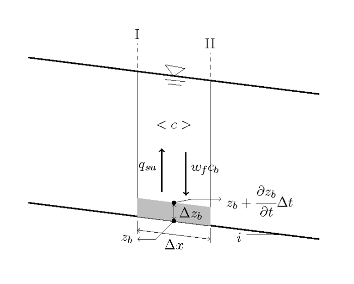
Figure 9.10 : Schematic of bed deformation from suspended sediment

(9.15)\[\cfrac{\partial z_b}{\partial t}= -\cfrac{1}{1-\lambda}(q_{su}-\alpha w_f <c>)\]

9.2.3. The Python codes

The Python code for the above calculation procedure is given here.

https://github.com/YasuShimizu/Bed-deformation-with-suspended-load

9.2.4. Calculation results

Figure 9.11 shows the results of calculations on the sedimentation of suspended sediment in a reservoir, using the above code. The calculation conditions are as follows: a bed gradient of \(i=1/700\), a channel length \(L\) of 10 km, the channel width \(B\) of 100 m, Manning’s roughness coefficient \(n\) of 0.02, a grain diameter of bed materials \(d\) of 0.1 mm, a discharge \(Q\) of 500 m \(^3\) /s flowing through a rectangular cross-section, and a water depth at the downstreamend \(H\) of 12 m. The conditions assume a dam reservoir. Note that this calculation example has the same conditions as the example for “Hydraulics for Field Work” (4) - suspended sediment and bed deformation- <http://mt.i-pn.jp/uploads/docs/suirigaku_old04_ver2006.pdf>`_ , and the calculation results are the same.

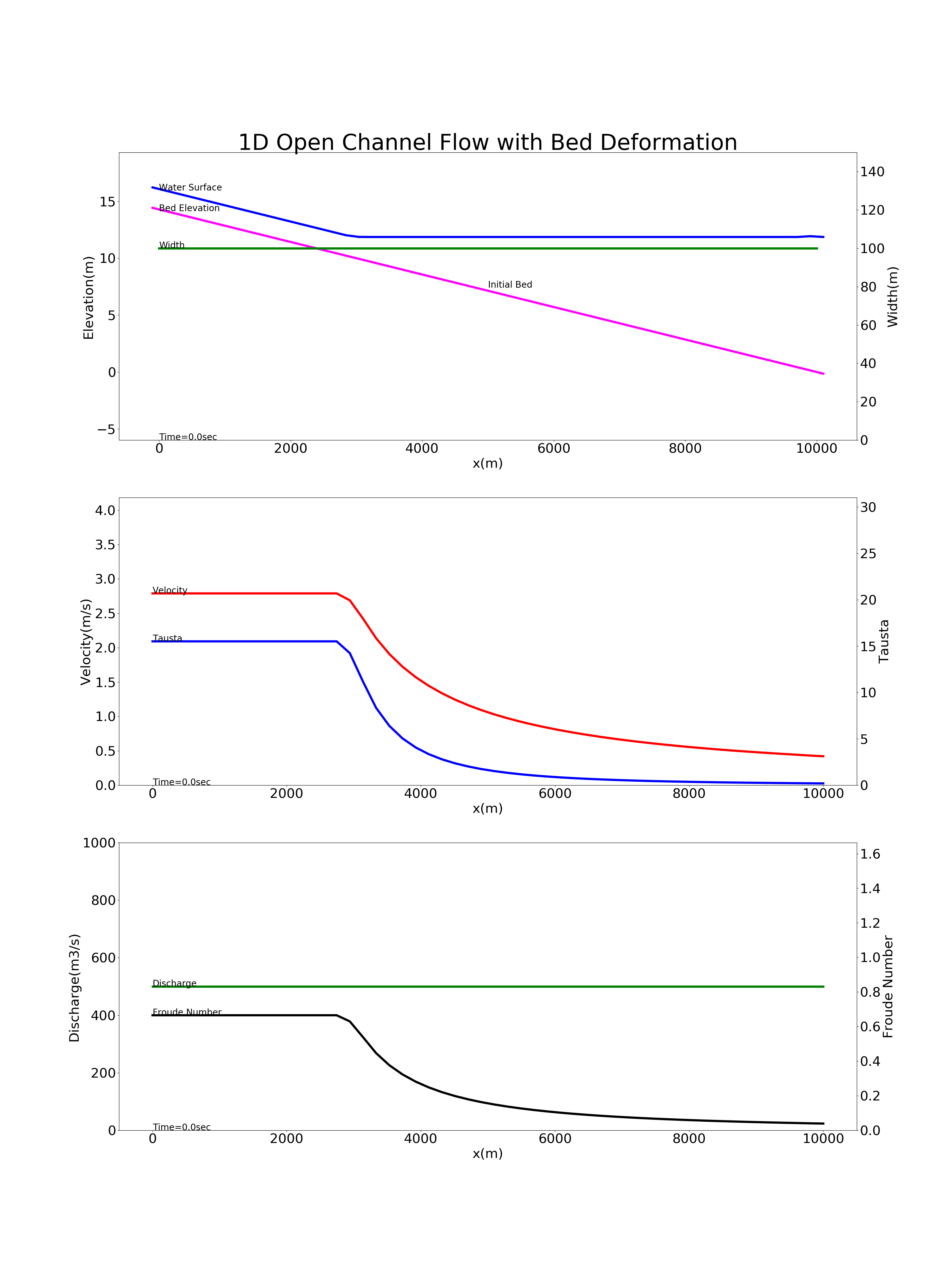
Figure 9.11 : Calculation for the deposition of suspended sediment in a reservoir