3. The higher-oder upwind difference scheme

3.1. Interpolation of variable distribution between grids

Let us assume that \(f(t)\) is the distribution of the variable, \(f\), of the triangular distribution at time \(t\), shown as the solid black line in Figure 3.1. and that the state of the advection of the distribution: a velocity of \(u(>0)\), and to the direction of \(x\). Also, at time \(t\), the vertex of triangle, or point \(A\), is assumed to be located at the \(i\) grid point. The distance of triangular distribution moved during the time, \(\Delta t\), is \(u \Delta t\). Therefore, the distribution supposed to move to the red broken line in the figure and the peak, or vertex, moves to the point \(A'\) shown by the red circle.

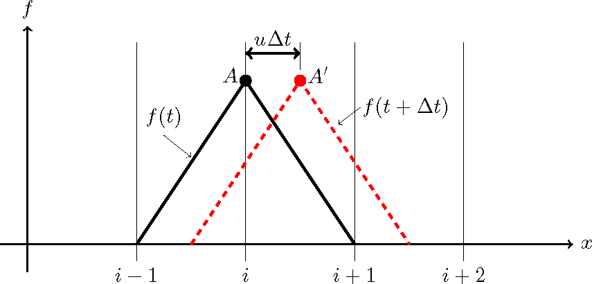
Figure 3.1 :: Advection of variable (1)

However, actually as shown by Figure 3.1, point \(A'\) is not on the calculation grid, but is in between the \(i\) th grid and \(i+1\) th grid. This means that we cannot express the triangular distribution that has moved and whose vertex is point \(A'\) with discrete values. When we try to express this with a conventional grid point, what we obtain is the shape shown by the blue line in Figure 3.2. The peak point \(A'\) can only be expressed as a shape whose peak has damped, such as point \(B_1\) or point \(B_2\). This is a graphic description of the numerical diffusion that was explained in Numerical diffusion caused by upwind differential shame of the previous chapter.

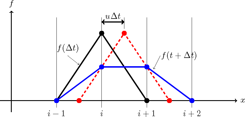
Figure 3.2 :: Advection of variable (2)

The above explanation is for the case where time moves from \(t\) to \(t+\Delta t\). Let us replace this with the case where time moves from \(t-\Delta t\) to \(t\). As shown in Figure 3.3, in order for the distribution of \(f\) at time \(t\) to be correctly represented as a triangular distribution whose peak is \(A\), it is necessary for the triangular distribution at time \(t-\Delta t\) with a peak of \(A'\) to be correctly expressed. However, because point \(A'\) is not on a grid point, it is impossible to express this shape by means of discrete values. This means that the shape of distribution at time \(t-\Delta t\) must not have discrete values but must have some form of a continuous function. This is the origin of the constrained interpolation profile (CIP) method explained as follows.

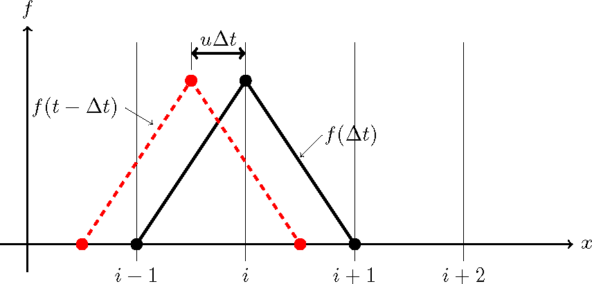
Figure 3.3 :: Advection of variable (3)

3.2. The basic concept of the CIP method

Let us review the 1D advection equation.

(3.1)\[\cfrac{\partial f}{\partial t}+u\cfrac{\partial f}{\partial x}=0\]

In (2.1) of the previous chapter, the advection velocity was expressed as \(c\), but here we express it as \(u\).

(There is no special reason for this change of expression. However, because \(u, v, w\) are often used for expressing flow velocity, here, we use \(u\).)

The numerical calculation of the 1D advection equation in Equation (3.1) has the same meaning as the estimation of \(f(x,t+\Delta t)\). As was explained in the previous section, the normal upwind difference scheme is applied to estimate by using \(f(x-\Delta x,t)\) and \(f(x,t)\) As mentioned above, this method provides a stable calculation, but it is not accurate because the calculation results diffuse (numerical diffusion). Here, I introduce the constrained interpolation profile method (the CIP method) developed by Yebe, et al. [Ref:1]. This higher-order difference scheme replaces the 1D upwind difference scheme.

Originally Equation (3.1) means that the distribution profile of variable \(f\) is conveyed at a speed of \(u\). Therefore, the distance of movement of the distribution profile, \(f\), during the time, \(\Delta t\), should be \(u \Delta t\). This means that the future \(f=f(x, t+\Delta t)\) should be the same as the current \(f=f(x-u\Delta t, t)\) (Refer to Figure 3.4).

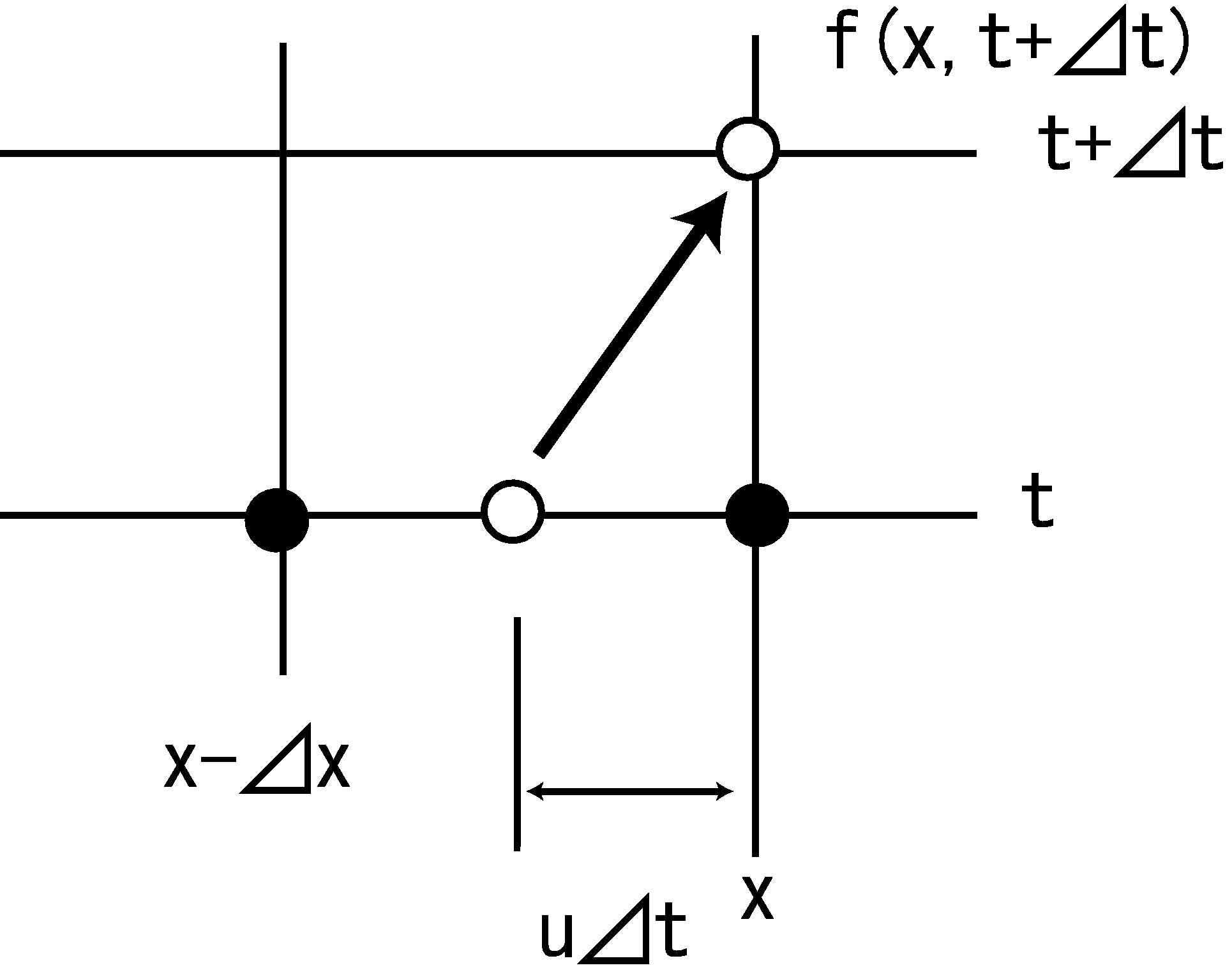
Figure 3.4 Conveying :\(f(x,t+\Delta t)\)

Instead of estimating the future \(f(x,t+\Delta t)\), if we can estimate the current \(f(x-u\Delta t, t)\), that value can be used as an estimate of the future value. This can be expressed by the following formula.

(3.2)\[f(x,t+\Delta t) \simeq f(x-u\Delta t, t)\]

3.3. Method for estimating the variable distribution form between grids

3.3.1. Introduction of a 3rd order function

There are many methods for estimating \(f(x-u\Delta t, t)\). The issue is that because \(f\) is given as discrete values, the known quantity of \(f\) is the point, ● of Figure 3.4. From the two ● points, \(f(x-u\Delta t, t)\) of ○ needs to be estimated. The simplest method is linking the two dots by a line and proportionally allocating the quantity. However, when \(f\) rapidly changes or when it increases and decreases between the two points, it is natural to express the estimated value by using a 3rd order function.

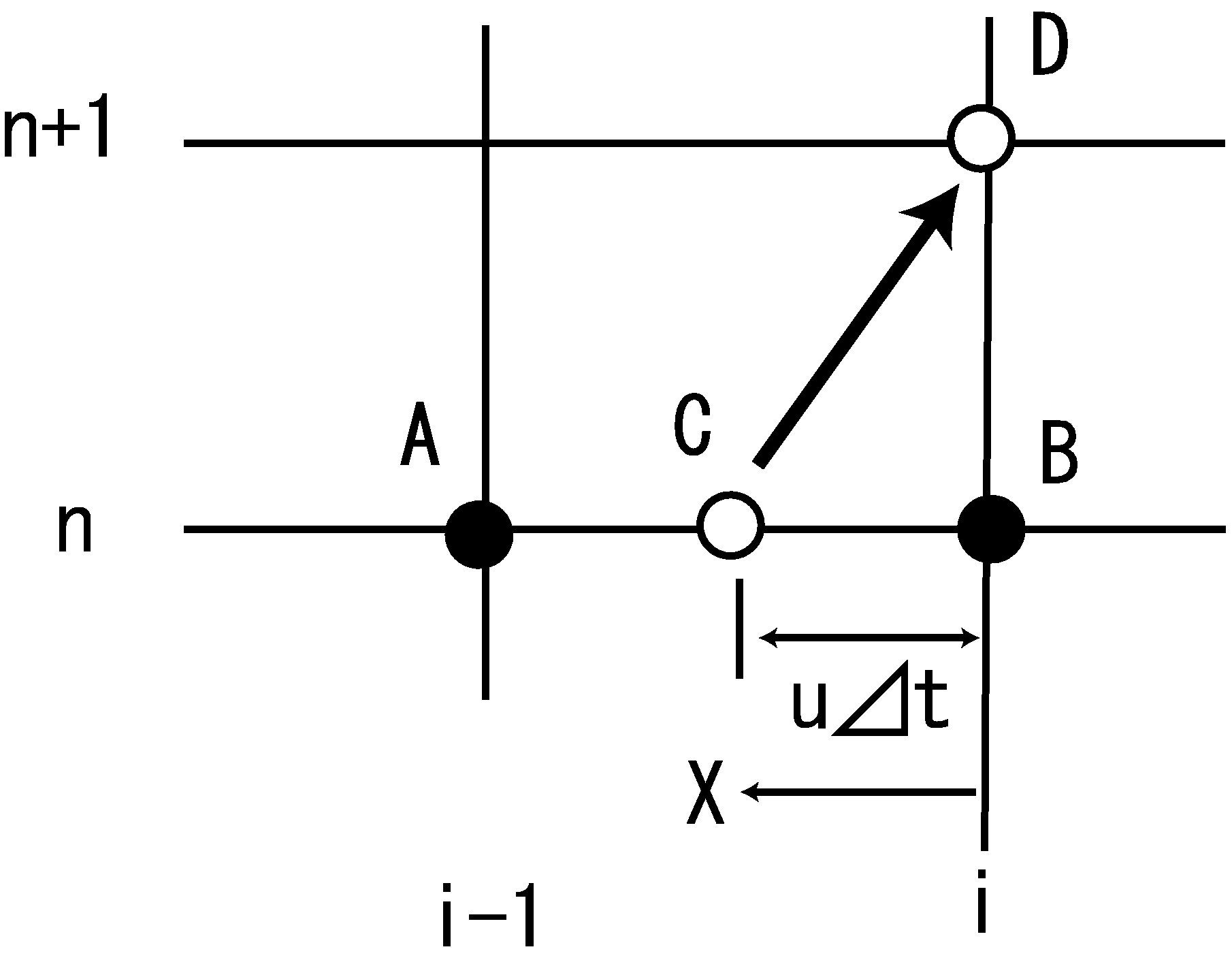
Figure 3.5 : Schematic diagram of the CIP method

As shown by Figure 3.5 discrete values are expressed in the direction of \(x\) as \(i\) and in the direction of \(t\) as \(n\). We denote \(f\) at points A and B as \(f(i-1,n)\) and \(f(i,n)\). Assuming that the distribution of \(f\) between A and B is expressed as a 3rd order function and that the distance from B to A is expressed as \(X\), then we have…

(3.3)\[F=a_1 X^3 + a_2 X^2 + a_3 X + a_4\]

This is a 3rd order function that has four parameters, \(a_1 \sim a_4\). Here, note that \(f\) gives discrete values defined for each grid point, while \(F\) is a 3D continuous function that interpolates \(f\) of each grid point between the grids. To determine the four parameters in Equation (3.3), the following four conditions are necessary. Two of them are given by…

(3.4)\[\begin{split}\mbox{at point B:} & F_{(X=0)}=f(i,n) \\ \mbox{at point A:} & F_{(X=\Delta x)} = f(i-1,n)\end{split}\]

What about the remaining two conditions? We can think about them in many ways (for example, by using \(f(i-2,n)\) or \(f(i+1,n)\)). In the CIP method, we use the gradient of \(f\) in the direction of the \(x\) axis. Thus,

(3.5)\[\begin{split}\mbox{at B:} & \displaystyle{{\partial F}\over{\partial x}}_{(X=0)}= {{\partial f}\over{\partial x}} (i,n) \\ \mbox{at A:} & \displaystyle{{\partial F}\over{\partial x}}_{(X=\Delta x)} = {{\partial f}\over{\partial x}}(i-1,n)\end{split}\]

By using equations (3.4) \(\sim\)(3.5), only with information given by \(i\) and \(i-1\), \(F\), the distribution of \(f\) between A and B can be estimated. This is one of the major advantages of the CIP method.

Equation (3.3) and its partial differentiation in terms of \(x\) are…

(3.6)\[F_x= {{\partial F}\over{\partial x}} =3 a_1 X^2 + 2 a_2 X +a_3\]

For the above equation, by applying the four conditions of equations (3.4) \(\sim\) (3.5), we can determine the parameters, \(a_1 \sim a_4\), and obtain \(F\). However, it seems a little complicated. Then, among equations (3.4) \(\sim\) (3.5), the conditions of point B (\(X=0\)) automatically satisfied by

(3.7)\[F(X)=\left[ (aX + b)X + f_x(i,n) \right] X + f(i,n)\]

Now, let us use this equation. Note that

(3.8)\[f_x(i,n) = \displaystyle{{\partial f}\over{\partial x}} (i,n)\]

Convert Equation (3.7) to

(3.9)\[F(X)=aX^3+bX^2+f_x(i,n)X+f(i,n)\]

And when we perform the partial differential in terms of \(x\), we have…

(3.10)\[F_x(X)=3aX^2+2bX+f_x(i,n)\]

Equation (3.9) and Equation (3.10) automatically satisfy the conditions of point B (\(X=0\)) of Equation (3.4) and Equation (3.5). Now, let us apply the conditions of point B (\(X=\Delta x\)) of Equation (3.4) and Equation (3.5) to Equation (3.9) and Equation (3.10). Then, we obtain…

(3.11)\[\begin{split}a\Delta x^3 + b \Delta x^2 + f_x(i,n) \Delta x + f(i,n) = f(i-1,n) \\ 3a\Delta x^2 + 2b\Delta x + f_x(i,n) = f_x(i-1,n)\end{split}\]

Therefore, we obtain…

(3.12)\[\begin{split}a=\displaystyle{{ \left[(f_x(i-1,n)+f_x(i,n) \right] \Delta x + 2 \left[f(i,n)-f(i-1,n) \right] }\over{\Delta x^3}} \\ b=\displaystyle{{ 3\left[(f(i-1,n)-f(i,n) \right]- \left[f_x(i-1,n)+2f_x(i,n) \right] \Delta x }\over{\Delta x^2}}\end{split}\]

3.3.1.1. Problem (1)

Drive Equation (3.12).

3.3.2. Summary of a method for estimating the distribution equation of link variables by using the CIP method.

In summary, the procedure for applying the CIP method to Equation (3.1) in order to obtain \(f(x,t+\Delta t)\) is as follows.

1. Obtain \(a, b\) for Equation (3.12).

2. Substitute \(a, b\) into Equation (3.7) to transform it to \(X=u\Delta t\) so as to obtain \(F(X=u\Delta t)=f(x-u\Delta t, t)\).

3. At the same time, use Equation (3.10) to obtain \(F_x(X=u\Delta t)=f_x(x-u\Delta t, t)\).

4. Obtain \(f(x,t+\Delta t)\) for Equation (3.2).

Execute this procedure for \(i=1 \sim N_i\), and when it finishes, update the time.

3.3.3. The Python code and calculation examples

An example Python code for the numerical solution of the 1D advection equation by the CIP method is given here. https://github.com/YasuShimizu/Python-Code/blob/main/cip.py

Performing this calculation yields the following results. Where, \(x_b\) = 10, \(x_p\) = 10, \(f_p\) = 0.5, \(u\) = 0.5．

Figure 3.6 : The 1D advection equation (CIP method)

The CIP method can thus be used to calculate how the triangular distribution in the initial conditions is not disrupted, and how it moves downstream at a constant speed. The results are almost identical to the theoretical solution (Figure 1) in the Appendix.

3.4. Advection equations with varying advection directions

Whereas The basic concept of the CIP method above described a calculation method for the case of constant advection direction, this section describes a method for the case where the advection direction varies. In the 1D advection equation, (3.1), the advection velocity, \(u\), was treated as constant in the previous explanations. Here, \(u\) is not a constant, but is a quantity that varies temporally and spatially. In general, in fluid, \(u\) is positive or negative depending on the direction of flow. The algorithm must be able to cope with both \(u>0\) and \(u<0\).

3.4.1. When u<0,

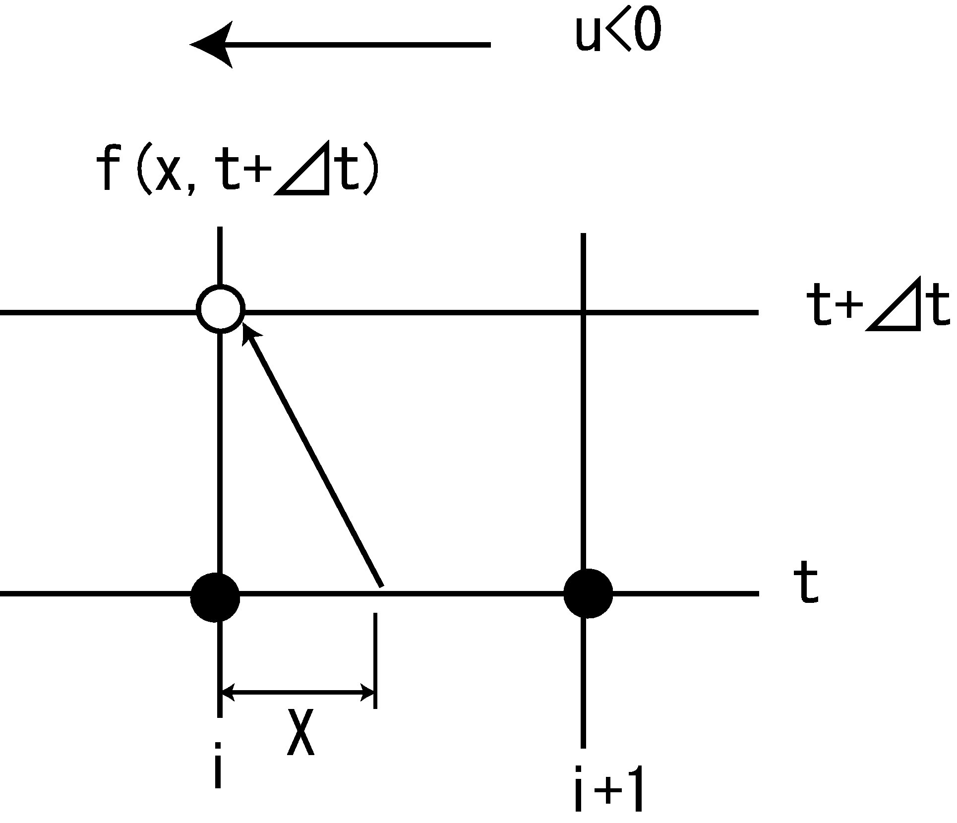
Figure 3.7 : Schematic for when \(u<0\).

As shown in the above figure, when \(u<0\), we assume that…

(3.13)\[X=-u\Delta t\]

and that the distribution of \(f\) between \(i\) and \(i+1\) is expressed with the following equation. Where, \(X>0\).

(3.14)\[F(X)=\left[ (aX + b)X + f_x(i) \right] X + f(i)\]

Here, the differentiation of \(F(X)\) is

(3.15)\[F'(X)=3aX^2+2bX+f_x(i)\]

Where, \(f_x\) is

(3.16)\[f_x = {{\partial f}\over{\partial x}}\]

\(F\) and \(F'\) derive from the conditions of…

(3.17)\[\begin{split}X=0 \mbox{: } & F(X)=f(i) \mbox{ and } F'(X)=f_x(i) \\ X=\Delta x \mbox{: } & F(X)=f(i+1) \mbox{ and } F'(X)=f'(i+1)\end{split}\]

as follows.

(3.18)\[\begin{split}a=\displaystyle{{ \left[(f_x(i+1)+f_x(i) \right] \Delta x + 2 \left[f(i)-f(i+1) \right] }\over{\Delta x^3}} \\ b=\displaystyle{{ 3\left[(f(i+1)-f(i) \right]- \left[f_x(i+1)+2f_x(i) \right] \Delta x }\over{\Delta x^2}}\end{split}\]

3.4.1.1. Problem (2)

Drive Formula (3.18).

3.4.2. When u>0,

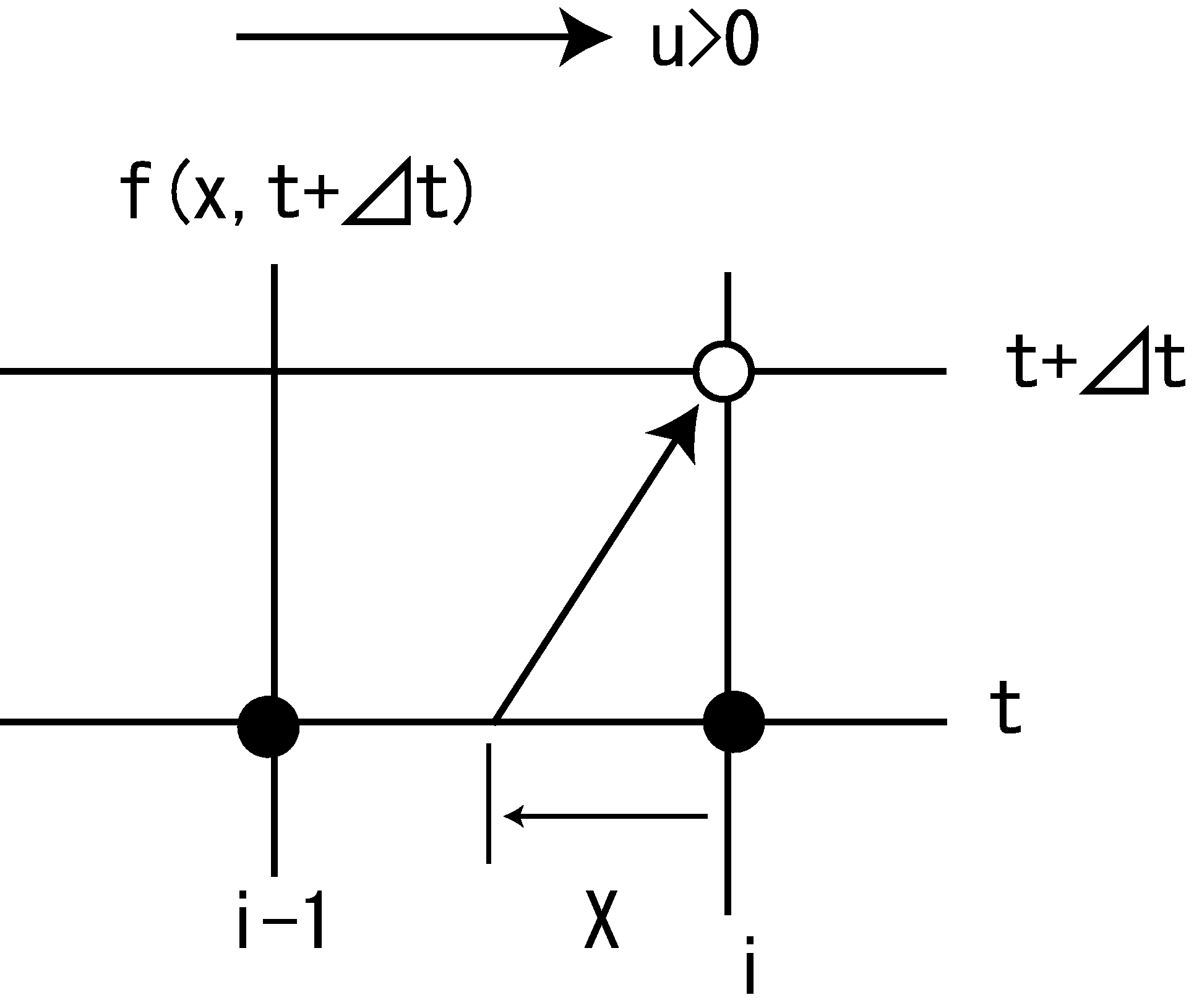
Figure 3.8 : Schematic diagram for when \(u>0\)

As shown in the above figure, when \(u>0\), we assume that…

(3.19)\[X = - u \Delta t\]

Then, despite the assumption that \(X = u \Delta t (>0)\) in the previous section, here, we assume u such that \(X<0\), as in (3.19). The reasons will be explained later, but the assumption enables us to use the same algorithm regardless of whether \(u<0\) or \(u>0\). For \(u>0\), the distribution of \(f\) between \(i\) and \(i-1\) is expressed by the following equation. This is completely the same form as Equation (3.14).

(3.20)\[F(X)=\left[ (aX + b)X + f_x(i) \right] X + f(i)\]

Then, the differentiation of \(F(X)\) is expressed as follows.

(3.21)\[F'(X)=3aX^2+2bX+f_x(i)\]

From the following conditions,

(3.22)\[\begin{split}X=0 \mbox{: } & F(X)=f(i) \mbox{ and } F'(X)=f_x(i) \\ X= -\Delta x \mbox{t: } & F(X)=f(i-1) \mbox{ and } F'(X)=f'(i-1).\end{split}\]

\(F\) and \(F'\) give the following formulas.

(3.23)\[\begin{split}a=\displaystyle{{ \left[(f_x(i-1)+f_x(i) \right] \Delta x - 2 \left[f(i)-f(i-1) \right] }\over{\Delta x^3}} \\ b=\displaystyle{{ 3\left[(f(i-1)-f(i) \right]+ \left[f_x(i-1)+2f_x(i) \right] \Delta x }\over{\Delta x^2}}\end{split}\]

3.4.2.1. Problem (3)

Drive Formula (3.23).

3.4.3. How can we make it usable for both u>0 and u<0?

Formula (3.18) is when \(u<0\), and Formula (3.23) is when \(u>0\).

These pairs are very similar. Then, we use the sign function (also known as the signal function or the signum function) that is defined as follows.

(3.24)\[\begin{split}\mbox {sign}(Y) & =1 & ,Y>0 \\ \mbox {sign}(Y) & =-1 & ,Y<0\end{split}\]

In addition, we define \(i_m\) as follows.

(3.25)\[i_m = i - \mbox{sign}(u)\]

Then, we have…

(3.26)\[\begin{split}u>0 \mbox{: } i_m & = i-1 \\ u<0 \mbox{: } i_m & = i+1\end{split}\]

Therefore, by assuming the following equations, instead of Equation (3.18) and Equation (3.23)…

(3.27)\[\begin{split}a=\displaystyle{{ \left[(f_x(i_m)+f_x(i) \right] \Delta x \cdot \mbox{sign}(u)- 2 \left[f(i)-f(i_m) \right] }\over{\Delta x^3 \cdot \mbox{sign}(u)}}\\ b=\displaystyle{{ 3\left[(f(i_m)-f(i) \right]+ \left[f_x(i_m)+2f_x(i) \right] \Delta x \cdot \mbox{sign}(u)}\over{\Delta x^2}}\end{split}\]

Then, we can use the same equations as for when \(u<0\) and for when \(u>0\).

3.4.3.1. Example

Use the CIP method to calculate the 1D advection equation for the case where the advection velocity \(u\) exhibits simple harmonic motion in the positive or negative direction, expressed in the following equation.

The initial conditions are the same as those for Figure 2.3.

(3.28)\[u=u_0 \sin \left( \cfrac{2\pi}{T_l} t \right)\]

Where, \(u_0\) is the maximum value of the oscillatory flow velocity, and \(T_l\) is the period of the oscillatory flow velocity.

3.4.4. The Python code and calculation examples

When the advection direction of the advection equation oscillates positively and negatively, an example of the Python code for numerical calculation by means of the CIP method is below.

https://github.com/YasuShimizu/Python-Code/blob/main/cip_pm.py

With the code, assuming that \(u_0\) = 2.0, \(T_l\) = 100, \(x_b\) = 10, \(x_p\) = 20, and \(f_p\) = 0.5, then we have Figure 3.9, which shows the calculation result.

Figure 3.9 : Calculation results when the advection direction oscillates positively and negatively

3.5. An advection equation with the source term

This section describes the splitting method, which is indispensable when performing numerical calculations for fluids. Fluid equations rarely have zero on the right side, as in the Equation (3.1), and many have a value on the right side. This is generally expressed as follows.

(3.29)\[\cfrac{\partial f}{\partial t}+u\cfrac{\partial f}{\partial x}=G\]

For the equations of motion of a fluid, \(G\) includes various external forces (or source terms), such as the surface slope, the bed slope, the friction, etc. in short, it is other elements than the advection term.

For convenience, the Equation (3.29) is divided into the following two equations.

(3.30)\[{{\partial f}\over{\partial t}} = G\]

(3.31)\[{{\partial f}\over{\partial t}}+u{{\partial f}\over{\partial x}} = 0\]

\(f(t)\) and \(f(t+\Delta t)\) are set as \(f^n\) and \(f^{n+1}\), respectively.

The calculation of \(f^n \rightarrow f^{n+1}\) by Equation (3.29) is performed as follows.

First, we use Equation (3.30) to calculate \(f^n \rightarrow \widetilde{f}\).

Second, calculate \(\widetilde{f} \rightarrow f^{n+1}\) with Equation (3.31). This two-phase calculation is called the splitting method. Only after splitting the calculation like this, can the CIP method be applied in the form of Equation (3.31). These two phases are called the non-advection phase and the advection phase.

In the CIP method, in addition to the time variation of \(f\) the spatial differentiation amount, \(f_x\), represented by Equation (3.27) is always required. Therefore, we calculate the differentiation amounts at the same time, as follows. For the non-advection phase, \(\displaystyle{{{\partial f}\over{\partial x}}^n \rightarrow \widetilde{{\partial f}\over{\partial x}}}\), For the advection phase, \(\displaystyle{\widetilde{{\partial f}\over{\partial x}} \rightarrow {{\partial f}\over{\partial x}}^{n+1}}\) In this way, they are calculated separately in two phases.

The above is summarized below.

Table 3.1 Splitting method

Phase name	Equation used	Updating \(f\)	Updating \(\cfrac{\partial f}{\partial x}\)
[A] non-advection phase	\(\displaystyle{{\partial f}\over{\partial t}}=G\)	(a) \(f^n \rightarrow \widetilde{f}\)	(b) \(\displaystyle{{{\partial f}\over{\partial x}}^n \rightarrow \widetilde{{\partial f}\over{\partial x}}}\)
[B] advection phase	\(\displaystyle{{{\partial f}\over{\partial t}}+u{{\partial f}\over{\partial x}}}=0\)	(c) \(\widetilde{f} \rightarrow f^{n+1}\)	(d) \(\displaystyle{\widetilde{{\partial f}\over{\partial x}} \rightarrow {{\partial f}\over{\partial x}}^{n+1}}\)

A method for using the split-equations to calculation each phase is given below. In the following explanation, if it is necessary to show differences other than the advection term, then the central difference scheme with the highest possible accuracy should be used.

3.5.1. Non-advection phase

From Equation (3.30),

(3.32)\[{{\widetilde{f}-f^n}\over{\Delta t}} = G^n\]

(3.33)\[\widetilde{f} = f^n +G^n \Delta t\]

Assuming that the calculation point is \(i\), then at…

(3.34)\[\widetilde{f}(i) = f^n(i) +G^n(i) \Delta t\]

\(f\) of the non-advection phase is updated (\(f^n \rightarrow \widetilde{f}\)).

We differentiate both sides of (3.33) with respect to \(x\), then we have…

(3.35)\[\widetilde{{\partial f}\over{\partial x}} ={{\partial f}\over{\partial x}}^n +{{\partial G}\over{\partial x}}^n \Delta t\]

Expressing \(\displaystyle{{{\partial G}\over{\partial x}}^n}\) in the above equation with the central difference scheme give us…

(3.36)\[\widetilde{{\partial f}\over{\partial x}} ={{\partial f}\over{\partial x}}^n +{{G^n(i+1)-G^n(i-1)}\over{2\Delta x}} \Delta t\]

Then, because of Equation (3.34), we have…

(3.37)\[\begin{split}G^n(i+1)={{\widetilde{f}(i+1)-f^n(i+1)}\over{\Delta t}} \\ G(i-1)={{\widetilde{f}(i-1)-f^n(i-1)}\over{\Delta t}}\end{split}\]

Here, let us substitute (3.37) into (3.36). Then, we have…

(3.38)\[\widetilde{{\partial f}\over{\partial x}}(i)={{\partial f}\over{\partial x}}^n(i)+{{1}\over{2\Delta x}} \left[\widetilde{f}(i+1)-f^n(i+1)-\widetilde{f}(i-1)+f^n(i-1)\right]\]

Therefore, updates of variables, \(f\), and their spatial differentiation amount, \(\displaystyle{{{\partial f}\over{\partial x}}}\), in the non-advection phase can be obtained as follows. (a) in Table Table 3.1 is given by Equation (3.34), and (b) in Table Table 3.1 is given by Equation (3.38).

3.5.2. Advection phase

Updating \(f\) is performed in (c) of Table Table 3.1. The CIP methods described so far can be applied without modification. That means that we apply Equation (3.14) or Equation (3.20) (they are the same), then we have…

(3.39)\[{f(i)}^{n+1}=F(X)= \left[(aX+b)X+ \widetilde{{\partial f}\over{\partial x}}(i) \right] X +\widetilde{f}(i)\]

Where, \(a\) and \(b\) are given by Equation (3.27).

Next is a method for updating the spatial differentiation amount, \(\displaystyle{{\partial f}\over{\partial x}}\), of the advection phase [(d) in the table Table 3.1]. Perform partial differentiation on both sides of Equation (3.31) with respect to \(x\).

(3.40)\[{{\partial \over \partial x}}\left( {{\partial f}\over{\partial t}} \right) + {{\partial \over \partial x}} \left( u {{\partial f}\over{\partial x}} \right) =0\]

Where, we assume that \(\displaystyle{{\partial f}\over{\partial x}}\) is \(f'\). And develop the second term. Then, we have

(3.41)\[{{\partial f'}\over{\partial t}} + u{{\partial f'}\over{\partial x}} = -{{\partial u}\over{\partial x}} f'\]

What we are doing here is updating \(\displaystyle{{\partial f}\over{\partial x}}\) in the advection phase. What we need to do is to use this equation to simply perform \(\widetilde{f'} \rightarrow {f'}^{n+1} \left( \displaystyle{ \widetilde{{\partial f}\over{\partial x}} \rightarrow {{\partial f}\over{\partial x}}^{n+1}} \right)\).

Now, let us compare Equation (3.40) and Equation (3.29). Equation (3.41) is equivalent to Equation (3.29) when substituting its \(f\) with \(f'\) and \(G\) with \(\displaystyle{-{{\partial u}\over{\partial x}} f'}\). As we did for Equation (3.29), we apply the splitting method to Equation (3.40). Therefore, we split the (3.40) into…

(3.42)\[{{\partial f'}\over{\partial t}} + u{{\partial f'}\over{\partial x}} = 0\]

(3.43)\[{{\partial f'}\over{\partial t}} = -{{\partial u}\over{\partial x}} f'\]

Assuming a middle value, \(\widehat{f'}\),　between \(\widetilde{f'}\) and \({f'}^{n+1}\), we calculate \(\widetilde{f'} \rightarrow \widehat{f'}\) with Equation (3.42), and \(\widehat{f'} \rightarrow {f'}^{n+1}\) with Equation (3.43).

One is to calculate Equation (3.42) by using the CIP method again. However, it seems better to use either Equation (3.15) (the spatial differentiation amount of \(F(X)\) ) or Equation (3.21) (also the spatial differentiation amount of \(F(X)\) ), which are used in the CIP method. (Equation (3.15) and Equation (3.21) have the same form.) Therefore, assuming that…

(3.44)\[\widehat{f'}(i) = \widetilde{F'}(X)\]

and calculate with

(3.45)\[\widehat{f'}(i) = 3aX^2 + 2bX + \widetilde{f'}(i)\]

Then, we apply the central difference scheme for Equation (3.43), and we have…

(3.46)\[{{{f'}^{n+1}(i) - \widehat{f'}(i)}\over{\Delta t}} = - {{u(i+1)-u(i-1))}\over{2\Delta x}} \widehat{f'}(i)\]

Consequently, we calculate using the following formula.

(3.47)\[{f'}^{n+1}(i) = \widehat{f'}(i) -{{u(i+1)-u(i-1))}\over{2\Delta x}} \widehat{f'}(i) \Delta t\]

3.5.2.1. Problem (4)

When \(G\) on the right side of Equation (3.29) is \(\displaystyle{D{{\partial^2 f}\over{\partial x^2}}}\),

\[\displaystyle{{{\partial f}\over{\partial t}}+u{{\partial f}\over{\partial x}}= D{{\partial^2 f}\over{\partial x^2}}}\]

it becomes an advection and diffusion equation. Describe the method to calculate this with the splitting method.

3.5.3. The Python code and calculation examples

You can find an example of the Python code for calculating advection-diffusion equations at…

https://github.com/YasuShimizu/Python-Code/blob/main/cip_pm_diffusion.py

With the code, now assuming that the diffusion coefficient \(D=0.5\) = 0.5, \(u_0\) = 2.0, and \(T_l\) = 100, then the calculation results is shown in Figure 3.10. It shows how the initially triangular distribution gradually becomes more diffuse as it moves from left to right, and vice versa.

Figure 3.10 : Advection-diffusion equation calculation results when the advection velocity oscillates positively and negatively

A number of high-precision difference methods have been proposed for advection terms, in addition to the CIP method, some of which are presented in the Appendix (Other higher-order difference schemes for the advection term).