Appendix V (The main flow and the secondary flow velocity distribution by Engelund [Ref:38]
Note
The formula was originally published by Engelund [Ref:38] Iwasaki Toshiki of Hokkaido University, who developed and rearranged the formula kindly provided the result for use in this text, and I further arranged it for the text.
This
Vertical velocity distribution of the main flow
Assuming that the direction of the depth-averaged flow is \(s\) , and that the direction of the vertical upward flow is \(z\) , then the motion of equation for uniform flow in the direction of \(s\) is given as follows.
(135) \[0=-g{{\partial H}\over{\partial s}}+{\partial \over{\partial z}} \left(\nu_t{{\partial u_s}\over{\partial z}}\right)\]
Where, \(g\) is the gravitational acceleration, \(H\) is the water level, \(s\) is the direction of the main downstreamward flow, \(u_s\) is the flow velocity in the \(s\) direction, \(z\) is the vertical coordinate axis, and \(\nu_t\) is the turbulent eddy viscosity.
The vertical distance is made dimensionless in terms of the water depth, \(h\) , and assuming that the riverbed elevation is \(z_b\) , then the dimensionless vertical distance, \(\zeta\) (0 at the riverbed and 1 at the water surface), is expressed as follows.
(136) \[\zeta=\cfrac{z-z_b}{h}\]
Assuming uniform flow and an energy gradient (= surface slope) of \(I_e\) , then \(I_e\) is expressed as follows.
(137) \[I_e=-{{\partial H}\over{\partial s}}\]
The depth-averaged velocity of the main flow, \(<u_s>\) , is expressed as follows.
(138) \[u_s(\zeta)=<u_s>f_s(\zeta)\]
Then, let us substitute f_s into the equation of motion, (135) .
This gives us…
(139) \[\cfrac{\partial^2 f_s}{\partial \zeta^2}=-\cfrac{gI_eh^2}{\nu_t <u_s>}\]
Integrate it with \(\zeta\) , which gives us…
(140) \[{{\partial f_s}\over{\partial \zeta}}=-\cfrac{gI_eh^2}{\nu_t<u_s>}\zeta+C_1\]
Where, \(C_1\) is the integration constant. Because the shear force is zero at the water surface, when \(\zeta=1\) we have \(C_1\) .
Therefore, \(C_1\) is the following equation.
Let us call it \(\beta\) , which gives us…
(141) \[C_1=\cfrac{gI_eh^2}{\nu_t<u_s>} \equiv \beta\]
Equation (140) is as follows.
(142) \[{{\partial f_s}\over{\partial \zeta}}=\beta(1-\zeta)\]
Then, integrate it with respect to \(\zeta\) once again.
Assuming that \(C_2\) is the integration constant, \(f_s\) is as follows.
(143) \[f_s=\beta\left(\zeta-\cfrac{1}{2}\zeta^2\right)+C_2\]
From the definition of the mean velocity,
(144) \[\int_0^1 f_s d\zeta =1=
\left[
\beta\left(\cfrac{1}{2}\zeta^2-\cfrac{1}{6}\zeta^3\right)+C_2\zeta
\right]^1_0
=\cfrac{1}{3}\beta+C_2\]
Therefore,
(145) \[C_2=1-\cfrac{1}{3}\beta\]
Now, let this back into Equation (144) . This gives us the following equation.
(146) \[f_s=\left(-{1 \over 2}\zeta^2+\zeta-{1 \over 3}\right)\beta+1\]
Let us express the turbulent eddy viscosity as \(\nu_t=\alpha u_\ast h\) .
Because the friction velocity, \(u_\ast\) , is \(u_\ast=\sqrt{ghI_e}\) , we have…
(147) \[\beta=\cfrac{gI_eh^2}{\nu_t<u_s>}=\cfrac{gI_eh}{\alpha u_\ast <u_s>}=\cfrac{u_\ast}{\alpha<u_s>}\]
Now, assuming that the velocity at the bed bottom (the slip velocity) is \(u_s^b\) , then…
(148) \[u_s^b=<u_s>f_s(0)=-\cfrac{u_\ast}{3\alpha}+<u_s>\]
Therefore,
(149) \[\cfrac{<u_s>}{u_\ast} = \cfrac{u_s^b}{u_\ast}+\cfrac{1}{3\alpha}\]
(150) \[\cfrac{u_s^b}{u_\ast}=2+{{1}\over{\kappa}} \ln {{h}\over{k_s}} =r_\ast\]
is assumed. Then, we have…
(151) \[u_\ast^2h(1-\xi)=\alpha u_* h{{\partial u}\over{\partial \xi}}\]
Therefore,
(152) \[\cfrac{<u_s>}{u_\ast} = r_\ast+\cfrac{1}{3\alpha}\]
(153) \[\cfrac{u_\ast}{<u_s>}= \cfrac{1}{r_\ast + \cfrac{1}{3\alpha}}
=\cfrac{3\alpha}{3\alpha r_\ast +1}\]
Substituting this into Equation (146) give us…
(154) \[\beta=\left(\cfrac{3\alpha}{3\alpha r_\ast +1}\right)\cfrac{1}{\alpha}
=\cfrac{1}{\alpha r_\ast+\cfrac{1}{3}}\]
(155) \[\cfrac{1}{\beta} = \alpha r_\ast + \cfrac{1}{3}\]
Consequently,
(156) \[f_s=\left(
-\cfrac{1}{2}\zeta^2+\zeta-\cfrac{1}{3}\right)\beta+1
=\left(
-\cfrac{1}{2}\zeta^2+\zeta-\cfrac{1}{3}+\cfrac{1}{\beta}
\right)\beta
=\cfrac{\alpha r_\ast + \zeta - \cfrac{1}{2} \zeta^2}{\alpha r_\ast + \cfrac{1}{3}}\]
Here, assuming that \(r_\ast \alpha=\chi\) and \(\chi_1=\alpha r_\ast +\cfrac{1}{3}\) , we have…
(157) \[f_s=\cfrac{\chi+\zeta-\cfrac{\zeta^2}{2}}{\chi_1}\]
Therefore, \(u_s(\zeta)\) is expressed as follows.
(158) \[u_s(\zeta)=<u_s>\cfrac{\chi+\zeta-\cfrac{\zeta^2}{2}}{\chi_1}\]
Equation (158) is the vertical velocity distribution in the streamline direction and is called the parabolic distribution .
Velocity distributions of secondary flow
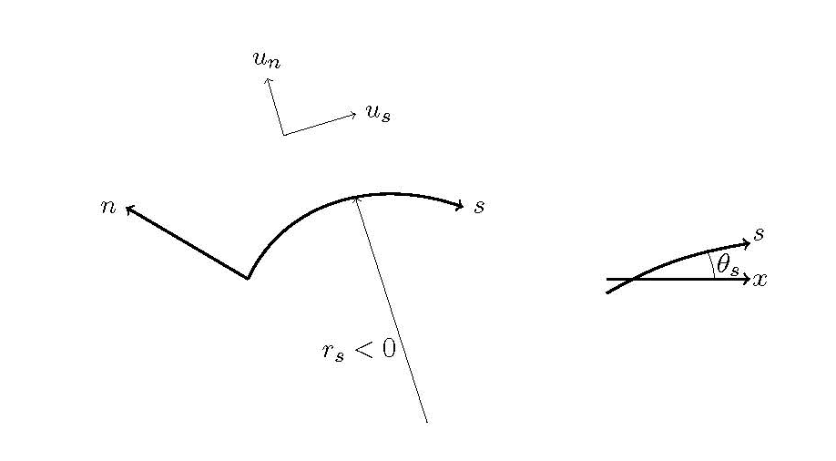
Figure 15 : Defining the coordinate system
As shown in Figure 15 \(r_s\) ,
(where, the \(s\) axis gives the direction of the main flow and \(r_s>0\) when the streamline of the main flow curves to the right against the \(s\) axis;
in Figure 15 \(r_s<0\) ), and when we assume that the \(n\) axis is perpendicular to the \(s\) axis and is positive on the left side toward \(s\) increases and that the direction of the flow velocity in the \(n\) direction is \(u_n\) , then the equation of motion for uniform flow in the \(n\) axis direction is given as follows.
(159) \[{{u_s^2}\over{r_s}} = -g{{\partial H}\over{\partial n}} +{{\partial}\over{\partial z}}
\left( \nu_t {{\partial u_n}\over{\partial z}} \right)\]
As you know…
(160) \[\cfrac{1}{r_s}= \cfrac{\partial \theta_s}{\partial s}\]
Where, \(\theta\) is the angle between the \(x\) axis and the main flow direction of the \(s\) axis.
Assuming the following distribution for the flow velocity in the \(n\) direction, then we have…
(161) \[u_n(\zeta)=A_n f_n(\zeta)\]
Where, \(A_n\) is the coefficient that expresses the secondary current intensity and \(f_n\) is the dimensionless flow velocity distribution function.
Substitute it into (159) and rearrange the formula, and we have…
(162) \[\cfrac{\partial^2 f_n}{\partial \zeta^2}=\cfrac{g h^2}{\nu_t A_n} \cfrac{\partial H}{\partial n}
+\cfrac{<u_s>^2 h^2}{\nu_t A_n r_s} f_s^2
=\cfrac{<u_s>^2h^2}{\nu_t A_n r_s} \left( \cfrac{g r_s}{<u_s>^2}\cfrac{\partial H}{\partial n}
+f_s^2 \right)\]
Now, let us define the following relationships.
(163) \[\cfrac{<u_s>^2h^2}{\nu_t A_n r_s} \equiv A\]
(164) \[\cfrac{g r_s}{<u_s>^2}\cfrac{\partial H}{\partial n} \equiv B\]
Then, Equation (162) can be rewritten as…
(165) \[\cfrac{\partial^2 f_n}{\partial \zeta^2}=A(B+f_s^2)\]
Integrating this with \(\zeta\) give us…
(166) \[\begin{split}\cfrac{\partial f_n}{\partial \zeta}
=AB\zeta+ A\int \left[\left\{{ {1}\over{\chi_1}}
\left( \chi + \zeta -{{1}\over{2}} \zeta^2 \right)\right\}^2
\right] d\zeta + C_3 \\
=AB \zeta + \cfrac{A}{{\chi_1}^2} \left[
\chi^2 \zeta + \chi \zeta^2 +{{1}\over{3}}(1-\chi)\zeta^3-{{1}\over{4}}\zeta^4+
{{1}\over{20}}\zeta^5 \right] +C_3\end{split}\]
Where, \(C_3\) is the constant of integration.
Because \(\cfrac{\partial f_n}{\partial \zeta}=0\) (= the slip condition) at the water surface, we have…
(167) \[C_3=-AB - \cfrac{A}{{\chi_1}^2} \left(\chi^2+{{2}\over{3}}\chi+{{2}\over{15}} \right)\]
Therefore,
(168) \[\begin{split}\cfrac{\partial f_n}{\partial \zeta}
=AB \zeta + \cfrac{A}{{\chi_1}^2} \left[
\chi^2 \zeta + \chi \zeta^2 +{{1}\over{3}}(1-\chi)\zeta^3-{{1}\over{4}}\zeta^4+
{{1}\over{20}}\zeta^5 \right] \\
-\left[
AB + \cfrac{A}{{\chi_1}^2} \left(\chi^2+{{2}\over{3}}\chi+{{2}\over{15}} \right)
\right]\end{split}\]
Integrating this once again with respect to \(\zeta\) give us…
(169) \[\begin{split}f_n={{1}\over{2}} AB\zeta^2 +\cfrac{A}{{\chi_1}^2} \left[
{{1}\over{2}}\chi^2 \zeta^2 + {{1}\over{3}}\chi \zeta^3 +{{1}\over{12}}(1-\chi)\zeta^4-{{1}\over{20}}\zeta^5+
{{1}\over{120}}\zeta^6 \right] \\
-\left[
AB + \cfrac{A}{{\chi_1}^2} \left(\chi^2+{{2}\over{3}}\chi+{{2}\over{15}} \right)
\right]\zeta + C_4\end{split}\]
Where, \(C_4\) is the constant of integration. The value of the integration in the depth-direction of the secondary flow is zero due to the definition of the secondary flow.
Therefore, because \(\displaystyle{\int_0^1 f_n d\zeta =0}\) …
(170) \[\begin{split}\int_0^1 f_n d \zeta =
{{1}\over{6}} AB\zeta^3 +\cfrac{A}{{\chi_1}^2} \left[
{{1}\over{6}}\chi^2 \zeta^3 + {{1}\over{12}}\chi \zeta^4 +{{1}\over{60}}(1-\chi)\zeta^5-{{1}\over{120}}\zeta^6+
{{1}\over{840}}\zeta^7 \right] \\
-\left[
AB + \cfrac{A}{{\chi_1}^2} \left(\chi^2+{{2}\over{3}}\chi+{{2}\over{15}} \right)
\right]\cfrac{\zeta^2}{2} + C_4\zeta =0\end{split}\]
Therefore, we obtain…
(171) \[C_4={{1}\over{3}}AB + \cfrac{A}{{\chi_1}^2} \left[
{{1}\over{3}} \chi^2 +{{4}\over{15}}\chi +{{2}\over{35}} \right]\]
Substituting this into Equation (169) give us…
(172) \[\begin{split}f_n={{A}\over{2}} \left(B+\cfrac{\chi^2}{{\chi_1}^2}\right)\zeta^2 +\cfrac{A}{{\chi_1}^2} \left[
{{1}\over{3}}\chi \zeta^3 +{{1}\over{12}}(1-\chi)\zeta^4-{{1}\over{20}}\zeta^5+
{{1}\over{120}}\zeta^6 \right] \\
-\left[
AB + \cfrac{A}{{\chi_1}^2} \left(\chi^2+{{2}\over{3}}\chi+{{2}\over{15}} \right)
\right]\zeta +{{1}\over{3}}AB+\cfrac{A}{{\chi_1}^2}
\left({{1}\over{3}}\chi^2+{{4}\over{15}}\chi+{{2}\over{35}}\right)\end{split}\]
Meanwhile, because the directions of the vector of bottom flow velocity and vector of shearing force are the same…
(173) \[\cfrac{u_n^b}{u_s^b} = \cfrac{\tau_n^b}{\tau_s^b}\]
Where, \(u_s^b, u_n^b, \tau_s^b, \tau_n^b\) are respectively the bottom flow velocities and the riverbed shear forces in the directions of \(s\) and \(n\) .
The respective values in Formula (173) are shown in (174) \(\sim\) (177) .
(174) \[u_s^b=<u_s>f_s(0)=<u_s> \cfrac{\chi}{\chi_1}\]
(175) \[u_n^b=A_n f_n(0) = A A_n \left[{{1}\over{3}}B + {{1}\over{{\chi_1}^2}} \left(
{{1}\over{3}}\chi^2+{{4}\over{15}}\chi+{{2}\over{35}} \right) \right]\]
(176) \[\cfrac{\tau_s^b}{\rho} = u_\ast^2\]
(177) \[\cfrac{\tau_n^b}{\rho} = \nu_t \left. \cfrac{\partial u_n}{\partial z} \right|_{z=0}
=\nu_t \cfrac{A_n}{h} \left. \cfrac{\partial f_n}{\partial \zeta} \right|_{\zeta=0}
=-\alpha u_\ast A_n A \left[
B+{{1}\over{{\chi_1}^2}} \left(\chi^2+{{2}\over{3}}\chi +{{2}\over{15}} \right) \right]\]
Substituting these into Equation (173) give us…
(178) \[\begin{split}\cfrac{ A A_n \left[\cfrac{1}{3}B + \cfrac{1}{{\chi_1}^2} \left(
\cfrac{1}{3}\chi^2+\cfrac{4}{15}\chi+\cfrac{2}{35} \right) \right]}
{<u_s> \cfrac{\chi}{\chi_1}} \\
=-\cfrac{\alpha u_\ast A_n A \left[
B+\cfrac{1}{{\chi_1}^2} \left(\chi^2+\cfrac{2}{3}\chi +\cfrac{2}{15} \right) \right]}
{u_\ast^2} \\
\cfrac{1}{3}B+\cfrac{1}{{\chi_1}^2} \left(
\cfrac{1}{3}\chi^2+\cfrac{4}{15}\chi+\cfrac{2}{35} \right) \\
=-\alpha \cfrac{<u_s>}{u_\ast} \cfrac{\chi}{\chi_1}
\left[
B+\cfrac{1}{{\chi_1}^2} \left(\chi^2+\cfrac{2}{3}\chi +\cfrac{2}{15} \right) \right]\end{split}\]
Here, let’s use the relationships of…
(179) \[\cfrac{<u_s>}{u_\ast} =
r_\ast +\cfrac{1}{3\alpha}=\cfrac{\chi_1}{\alpha}, \; \;
\chi_1=\chi+\cfrac{1}{3}\]
We have…
(180) \[\cfrac{1}{3}B+\cfrac{1}{{\chi_1}^2} \left(
\cfrac{1}{3}\chi^2+\cfrac{4}{15}\chi+\cfrac{2}{35} \right)
=-\chi \left[
B+\cfrac{1}{{\chi_1}^2} \left(\chi^2+\cfrac{2}{3}\chi +\cfrac{2}{15} \right) \right]\]
(181) \[\left(\chi+\cfrac{1}{3}\right)B=-\cfrac{1}{{\chi_1}^2}
\left(\chi^3+\chi^2+\cfrac{2}{5}\chi+\cfrac{2}{35}\right)\]
(182) \[B=-\cfrac{1}{{\chi_1}^3}\left(\chi^3+\chi^2+\cfrac{2}{5}\chi+\cfrac{2}{35}\right)\]
Therefore, \(f_n\) is…
(183) \[\begin{split}\cfrac{f_n}{A}=\cfrac{1}{2}\left(B+\cfrac{\chi^2}{{\chi_1}^2}\right)\zeta^2
+\cfrac{1}{{\chi_1}^2} \left[
\cfrac{1}{3}\chi\zeta^3+\cfrac{1}{12}(1-\chi)\zeta^4-\cfrac{1}{20}\zeta^5+\cfrac{1}{120}\zeta^6 \right] \\
-\left[B+\cfrac{1}{{\chi_1}^2}\left(\chi^2+\cfrac{2}{3}\chi+\cfrac{2}{15}\right)\right]\zeta
+\left[\cfrac{1}{3}B+\cfrac{1}{{\chi_1}^2}\left(\cfrac{1}{3}\chi^2+\cfrac{4}{15}\chi+\cfrac{2}{35}\right)\right]\end{split}\]
Now, when we apply the relationships of Equation (180) , the last term of the right side is…
(184) \[\begin{split}\cfrac{f_n}{A}=\cfrac{1}{2}\left(B+\cfrac{\chi^2}{{\chi_1}^2}\right)\zeta^2
+\cfrac{1}{{\chi_1}^2} \left[
\cfrac{1}{3}\chi\zeta^3+\cfrac{1}{12}(1-\chi)\zeta^4-\cfrac{1}{20}\zeta^5+\cfrac{1}{120}\zeta^6 \right] \\
-\left[B+\cfrac{1}{{\chi_1}^2}\left(\chi^2+\cfrac{2}{3}\chi+\cfrac{2}{15}\right)\right]\zeta
-\chi \left[
B+\cfrac{1}{{\chi_1}^2} \left(\chi^2+\cfrac{2}{3}\chi +\cfrac{2}{15} \right) \right] \\
=\cfrac{1}{{\chi_1}^2} \left[
-\left(\chi^2+\cfrac{2}{3}\chi+\cfrac{2}{15}\right) \left(\zeta+\chi\right)
+\cfrac{1}{2}\chi^2 \zeta^2+\cfrac{1}{3}\chi\zeta^3 \right. \\
+\left. \cfrac{1}{12}\left(1-\chi \right)\zeta^4-\cfrac{1}{20}\zeta^5+\cfrac{1}{120}\zeta^6
\right]+B\left(\cfrac{1}{2}\zeta^2-\zeta-\chi\right)\end{split}\]
Because…
(185) \[\begin{split}A=\cfrac{<u_s>^2 h^2}{\nu_t A_n r_s}=
\cfrac{1}{A_n} \cfrac{<u_s>^2 h^2}{\alpha u_\ast h r_s} \\
=\cfrac{1}{A_n} \cfrac{1}{\alpha} \cfrac{<u_s>}{u_\ast} <u_s> \cfrac{h}{r_s}
=\cfrac{1}{A_n} \cfrac{1}{C_f \chi_1} <u_s> \cfrac{h}{r_s}\end{split}\]
Let us define the secondary flow intensity, \(A_n\) , as follows.
(186) \[A_n = <u_s>\cfrac{h}{r_s}\]
Eventually, the distribution of the secondary flow is as follows.
(187) \[u_n=A_n f_n, \; \; f_n=\cfrac{G_0(\zeta)}{C_f \chi_1}\]
Where,
(188) \[\begin{split}G_0(\zeta)=\cfrac{1}{{\chi_1}^2}\left[
-\left(\chi^2+\cfrac{2}{3}\chi+\cfrac{2}{15}\right)\left(\zeta+\chi\right)+\cfrac{1}{2}\chi^2\zeta^2+\cfrac{1}{3}\chi\zeta^3 \right. \\
\left. +\cfrac{1}{12}\left(1-\chi\right)\zeta^4 -\cfrac{1}{20}\zeta^5+\cfrac{1}{120}\zeta^6 \right]+\chi_{20}\left(\cfrac{1}{2}\zeta^2-\zeta-\chi\right)\end{split}\]
(189) \[\chi_{20} = B = -\cfrac{1}{{\chi_1}^3} \left(\chi^3+\chi^2+\cfrac{2}{5}\chi+\cfrac{2}{35}\right), \: \: \cfrac{<u_s>}{u_\ast} = \cfrac{1}{\sqrt{C_f}}, \; \chi=\chi_1-\cfrac{1}{3}\]
This is Engelund’s 6th order formula for the secondary flow.
Bottom flow velocity
In the riverbed deformation calculation, the direction of the bottom velocity (the direction of sediment transport) that takes into account the secondary flow is important.
Now, let’s obtain the bottom flow velocity from the flow velocity distribution we have obtained thus far.
(190) \[\begin{split}\left. u_n\right|_{z=0}=A_n f_n(0) \\
=\cfrac{A_n}{C_f \chi_1} \left[
-\cfrac{\chi}{{\chi_1}^2}\left(\chi^2+\cfrac{2}{3}\chi+\cfrac{2}{15}\right)
+\cfrac{\chi}{{\chi_1}^3} \left(\chi^3+\chi^2+\cfrac{2}{5}\chi+\cfrac{2}{35}\right) \right] \\
=\cfrac{A_n \chi}{C_f {\chi_1}^4} \left[
\left(\chi^3+\chi^2+\cfrac{2}{5}\chi+\cfrac{2}{35}\right)
-\chi_1 \left(\chi^2+\cfrac{2}{3}\chi+\cfrac{2}{15}\right) \right] \\
=\cfrac{A_n \chi}{C_f {\chi_1}^4} \left[
\left(\chi^3+\chi^2+\cfrac{2}{5}\chi+\cfrac{2}{35}\right)
-\left( \chi + {1 \over 3} \right)\left(\chi^2+\cfrac{2}{3}\chi+\cfrac{2}{15}\right) \right] \\
=\cfrac{A_n \chi}{C_f {\chi_1}^4} \left(\cfrac{2}{45}\chi+\cfrac{4}{315}\right)\end{split}\]
Note that formulas for the bottom flow velocity in the transverse direction (\(n\) direction) that are generally used in 2D models are those such as such as…
(191) \[\left. u_n \right|_{z=0} = \left. u_s \right|_{z=0} N_\ast \cfrac{h}{r_s}\]
Such formulas tend to be expressed in relation to the bottom of the main flow direction (the \(s\) direction).
The bottom flow velocity of the main flow is…
(192) \[\left. u_n \right|_{z=0} = \cfrac{\chi}{\chi_1} N_\ast <u_s> \cfrac{h}{r_s}\]
Meanwhile, for Equation (190) , by giving the equilibrium state of \(A_n\) , we have…
(193) \[\left. u_n \right|_{z=0}
=\cfrac{A_n \chi}{C_f {\chi_1}^4} \left(\cfrac{2}{45}\chi+\cfrac{4}{315}\right)
=\cfrac{\chi}{C_f {\chi_1}^4} \left(\cfrac{2}{45}\chi+\cfrac{4}{315}\right)
<u_s>\cfrac{h}{r_s}\]
Now, by comparing Equation (192) and Equation (193) , we have…
(194) \[N_\ast =\cfrac{1}{C_f {\chi_1}^3} \left(\cfrac{2}{45}\chi + \cfrac{4}{315}\right)\]
Secondary flow intensity
For example, assuming \(\alpha=\cfrac{\kappa}{6}=0.077\) and \(C_f=0.01\) , we have \(N_\ast=7.03\) .
This is the basis of the secondary flow intensity \(N_\ast=7\) which is often used in the calculation of 2D riverbed deformation.”
In contrast, when \(N_\ast\) is given as the condition, we have…
(195) \[C_f =\cfrac{1}{N_\ast {\chi_1}^3} \left(\cfrac{2}{45}\chi + \cfrac{4}{315}\right)\]