Appendix I (Theory and basic formulas of flow and bed deformation calculation)

Theoretical solutions to advection equations

For the advection equation

(1)\[\cfrac{\partial f}{\partial t}+c\cfrac{\partial f}{\partial x}=0\]

perform the following variable conversions.

(2)\[\begin{split}X=x-ct \\ T= \; \; t.\end{split}\]

This is equivalent to set new coordinates \(X,T\) that move together with the origin moving at a velocity of \(c\). This means, for example, that we suppose we have a car moving at a speed of \(c\) in the original space, and we place coordinates in the car whose origin is on the \(X\) axis that moves with the car.

From Equation (2),

(3)\[\begin{split}\cfrac{\partial}{\partial x}=\cfrac{\partial X}{\partial x} \cfrac{\partial}{\partial X} +\cfrac{\partial T}{\partial x} \cfrac{\partial}{\partial T}\\ \cfrac{\partial}{\partial t}=\cfrac{\partial X}{\partial t} \cfrac{\partial}{\partial X} +\cfrac{\partial T}{\partial t} \cfrac{\partial}{\partial T}\end{split}\]

Where,

(4)\[\cfrac{\partial X}{\partial x}=1, \; \; \cfrac{\partial X}{\partial t}=0, \; \; \cfrac{\partial T}{\partial x}=1, \; \; \cfrac{\partial T}{\partial t}=0.\]

Therefore,

(5)\[\cfrac{\partial}{\partial x} = \cfrac{\partial}{\partial X}, \; \; \cfrac{\partial}{\partial t} = -c \cfrac{\partial}{\partial X} + \cfrac{\partial}{\partial T}\]

Substituting Equation (5) into Equation (1), we have…

(6)\[\cfrac{\partial f}{\partial t}+c\cfrac{\partial f}{\partial x} = -u\cfrac{\partial f}{\partial X} + \cfrac{\partial f}{\partial T} + u\cfrac{\partial f}{\partial X} = \cfrac{\partial f}{\partial T} =0\]

That is, in coordinates (\(X,T\)) moving at a speed of \(c\), we have…

(7)\[\cfrac{\partial f}{\partial T} =0 \; \; \; \mbox{or} \; \; \; f=\mbox{constant}\]

In other words, the distribution of \(f\) is kept constant while moving at a speed of \(c\). For example, when the initial distribution is triangular, the solutions to this equation maintain a triangle that is moving as shown in Figure 1.

Figure 1 : Theoretical solutions to advection equations

Other higher-order difference schemes for the advection term

When a typical difference method other than the CIP method is applied for the advection term, then its difference equation, Python codes, and calculation results are as below.

Kawamura-Kuwahara scheme (K-K scheme) [Ref:2]

Difference equation

(8)\[\begin{split}c\cfrac{\partial f}{\partial x} = c \cfrac{-f(i+2)+8\left\{f(i+1)-f(i-1)\right\}+f(i-2)}{12\Delta x} \\ +|c| \cfrac{f(i+2)-4f(i+1)+6f(i)-4f(i-1)+f(i-2)}{4\Delta x}\end{split}\]

Python codes

https://github.com/YasuShimizu/Python-Code/blob/main/kk.py

Calculation results

Figure 2 : K-K scheme

QUICK scheme [Ref:3]

Difference equation

(9)\[\begin{split}c\cfrac{\partial f}{\partial x} = c \cfrac{-f(i+2)+10\left\{f(i+1)-f(i-1)\right\}+f(i-2)}{16\Delta x} \\ +|c| \cfrac{f(i+2)-4f(i+1)+6f(i)-4f(i-1)+f(i-2)}{16\Delta x}\end{split}\]

Python codes

https://github.com/YasuShimizu/Python-Code/blob/main/quick.py

Calculation results

Figure 3 : QUICK scheme

A fifth-order upwind difference scheme [Ref:4]

Difference equation

(10)\[\begin{split}c\cfrac{\partial f}{\partial x} = c \cfrac{f(i+3)-9f(i+2)+45\left\{f(i+1)-f(i-1)\right\}+9f(i-2)-f(i-3)}{60\Delta x} \\ +|c| \cfrac{-f(i+3)+6f(i+2)-15f(i+1)+20f(i)-15f(i-1)+6f(i-2)-u(i-3)}{60\Delta x}\end{split}\]

Python codes

https://github.com/YasuShimizu/Python-Code/blob/main/od5th.py

Calculation results

Figure 4 : A fifth-order upwind difference scheme

Expressions of riverbed shear force

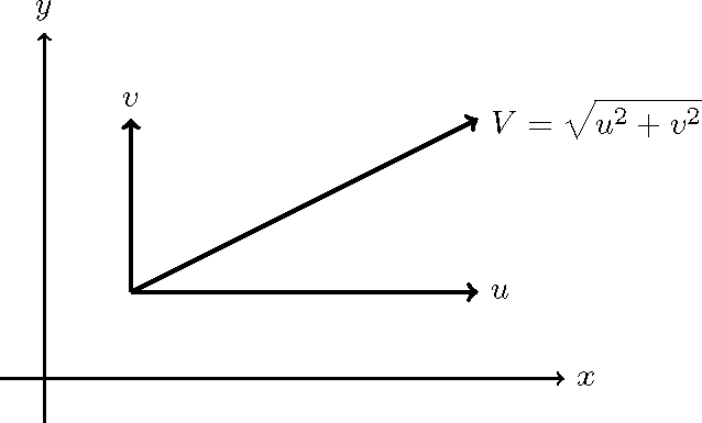
Figure 5 : Component indications of flow velocity

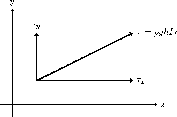
Figure 6 : Component indications of riverbed shear force

As shown in Figure 5 and Figure 6, the direction of the depth velocity and the direction of the riverbed shear force are assumed to coincide. The composite components, \(V=\sqrt{u^2+v^2}\), of the depth-averaged velocity can be expressed by Manning’s equation as follows.

(11)\[V={1 \over n_m} h^{2/3} I_e^{1/2}\]

Where, \(I_e\) is the energy gradient. Therefore, the riverbed shear force, \(\tau\), due to the composite velocity, \(V\), is…

(12)\[\tau=\rho g h I_e = {{\rho g n_m^2 V^2}\over{h^{1/3}}}\]

From Equation (12), Figure 5 and Figure 6, the representation of \(\tau\) separated in the \(x, y\) direction is as follows:

(13)\[\begin{split}\tau_x = \tau { u \over V} = {{\rho g n_m^2 u \sqrt{u^2+v^2}}\over h^{1/3}} \\ \tau_y = \tau { v \over V} = {{\rho g n_m^2 u \sqrt{u^2+v^2}}\over h^{1/3}}\end{split}\]

River bank (sidewall) friction resistance

In general, the shear force acting on a wall along the flow direction can be expressed by following equations, where \(c_w\) is the friction coefficient, \(\tau_w\) is the wall shear force, \(\rho\) is the fluid density, and \(u_w\) is the velocity along the wall.

(14)\[\cfrac{\tau_w}{\rho}=c_w u_w^2.\]

In order to match the direction of flow velocity (positive or negative) with the direction of shear force,

(15)\[\cfrac{\tau_w}{\rho}=c_w u_w |u_w|\]

are required to be satisfied.

The shear resistance of the riverbank (sidewall) in free-surface flow can be taken into account in the second derivative term with respect to \(y\) of the right-side diffusion term of the equation of motion in the \(x\) direction in Equation (7.8). Therefore…

(16)\[\cfrac{\partial}{\partial y}\left( \nu_t \cfrac{\partial u}{\partial y} \right) =\cfrac{\partial}{\partial y}\left(\cfrac{\tau_w}{\rho}\right) =\cfrac{1}{\Delta y}\left[ \left( \cfrac{\tau_w}{\rho} \right)_{y+} - \left( \cfrac{\tau_w}{\rho} \right)_{y-}\right].\]

Where, the subscripts \(y+\) and \(y-\) indicate the values on the \(+\) and \(-\) sides of the \(y\) axis.

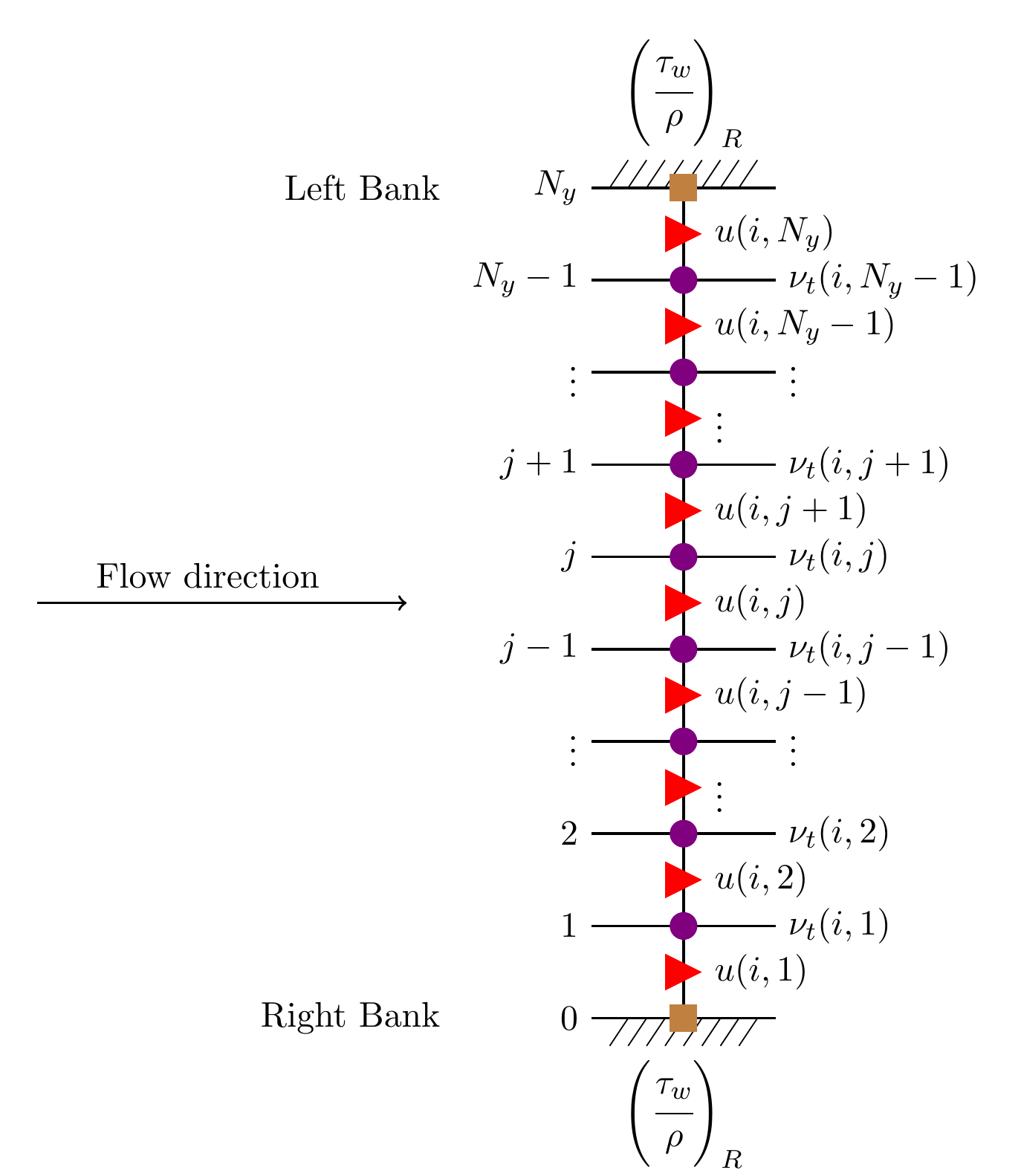
Figure 7 : Explanation of lateral shear stress and bank shear stress

Let us express the shear force along the \(x\) axis using the computational grid shown in Figure 7. For a channel other than a riverbank,

(17)\[\cfrac{\tau_w}{\rho}(i,j)=\cfrac{\nu_t(i,j)}{\Delta y} \left\{u(i,j+1)-u(i,j)\right\}\]

On the right bank, the relationship in Equation (15), gives us…

(18)\[\cfrac{\tau_w}{\rho}(i,0)=c_w u(i,1) |u(i,1)|\]

Similarly, for the left bank, we have…

(19)\[\cfrac{\tau_w}{\rho}(i,N_y)=c_w u(i,N_y) |u(i,N_y)|\]

Therefore, for a channel other than a riverbank,

(20)\[\cfrac{\partial}{\partial y}\left( \nu_t \cfrac{\partial u}{\partial y} \right) =\cfrac{1}{\Delta y}\left[\nu_t(i,j) \cfrac{u(i,j+1)-u(i,j)}{\Delta y}-\nu_t(i,j-1)\cfrac{u(i,j)-u(i,j-1)}{\Delta y} \right].\]

For the right bank,

(21)\[\cfrac{\partial}{\partial y}\left( \nu_t \cfrac{\partial u}{\partial y} \right) =\cfrac{1}{\Delta y}\left[\nu_t(i,1) \cfrac{u(i,2)-u(i,1)}{\Delta y}-c_w u(i,1)|u(i,1)|\right]\]

For the left bank,

(22)\[\cfrac{\partial}{\partial y}\left( \nu_t \cfrac{\partial u}{\partial y} \right) =\cfrac{1}{\Delta y}\left[c_w u(i,N_y)|u(i,N_y)| -\nu_t(i,N_y-1)\cfrac{u(i,N_y)-u(i,N_y-1)}{\Delta y}\right]\]

Wall friction coefficient

Assuming that the effect of bottom friction is relatively negligible near the sidewalls at some distance from the bottom,and that friction acts only from the sides, then the horizontal distribution of flow velocity in the downstream direction can be considered to follow a theoretical velocity distribution such as that of the logarithmic law in the horizontal direction. Applying the logarithmic law distribution equation in the vertical direction, Equation (41), to the horizontal direction, we obtain the following equation.

(23)\[\cfrac{u}{u_{\ast w}}=\cfrac{1}{\kappa}\log \cfrac{y}{y_0}\]

Where, \(u_{\ast w}\) is the friction velocity of the wall, \(\kappa\) is Karman’s universal constant, and \(y\) is the horizontal distance. \(y_0\) is the distance from the wall to the point where the flow velocity is zero, and when the wall is rough, applying Equation (64) below gives us…

(24)\[y_0=\cfrac{k_s}{30}\]

Also, expressing \(u_{\ast w}\) with the wall shear force of Equation (15) gives us…

(25)\[u_{\ast w}|u_{\ast w}|=\cfrac{\tau_w}{\rho}=c_w u_w |u_w|.\]

In the case of \(u_{\ast w} >0\), we have…

(26)\[{u_{\ast w}}^2 = c_2 {u_w}^2 \hspace{5mm} \mbox{or} \hspace{5mm} u_{\ast w}=\sqrt{c_w} u_w.\]

Let \(u_w\) be the velocity at the calculation point closest to the sidewall, and let \(y_1\) be the distance from that point to the sidewall. Then, we have…

(27)\[\cfrac{u_w}{u_{\ast w}}= \cfrac{1}{\kappa}\ln \cfrac{y_1}{y_0} = \cfrac{1}{\sqrt{c_w}}\]

Therefore,

(28)\[c_w= \cfrac{1}{\left( \cfrac{1}{\kappa}\ln \cfrac{y_1}{y_0}\right)^2}= \cfrac{\kappa^2}{\left( \ln \cfrac{30y_1}{k_s}\right)^2}\]

When the equivalent roughness height of the sidewall, \(k_s\), and the horizontal distance from the sidewall to the calculation point of the velocity that is closest to the sidewall, \(y_1\), are given, then Equation (27) is able to give \(c_w\) as a physical constant.

Velocity distribution

Here, we explain the vertical distribution of horizontal velocity.

Logarithmic velocity distribution (logarithmic law)

Distribution equation in the vertical direction

The equation of motion in the downstream direction for 1D steady flow is given by the following equation.

(29)\[0=-g\cfrac{\partial H}{\partial x}+\cfrac{\partial}{\partial z} \left(\nu_t \cfrac{\partial u}{\partial z}\right)\]

Where, \(u\) is the velocity in the downstream direction, \(g\) is the gravitational acceleration, \(H\) is the water level, \(x\) is the coordinate axis in the downstream direction, \(z\) is the vertical coordinate axis, and \(\nu_t\) is the eddy kinematic viscosity coefficient. Since the flow is uniform flow, we have \(-\cfrac{\partial H}{\partial x}=I_e\) (\(I_e\) is the energy gradient). Assuming that the riverbed elevation is \(z_b\) and the depth is \(h\), then the water level is \(H (=z_b+h)\), and we can define the dimensionless coordinates as

(30)\[\zeta=\cfrac{z-z_b}{h}\]

Then, from Equation (30) we have \(\partial z = h \partial \zeta\). Therefore, Equation (29) is

(31)\[0={u_\ast}^2+ \cfrac{\partial}{\partial \zeta} \left(\cfrac{\nu_t}{h} \cfrac{\partial u}{\partial \zeta}\right)\]

Where, \(u_\ast (=\sqrt{g h I_e})\) is the friction velocity. Let us integrate Equation (31) with \(\zeta\).

(32)\[{u_\ast}^2 \zeta + \left(\cfrac{\nu_t}{h} \cfrac{\partial u}{\partial \zeta}\right) + C_1 = 0\]

Where, \(C_1\) is the integration constant. Because the shear force is zero at the water surface, when \(\zeta=1\), we have \(\nu_t \cfrac{\partial u}{\partial \zeta}=0\). Consequently,

(33)\[C_1 = -{u_\ast}^2\]

Therefore, Equation (32) derives

(34)\[-{u_\ast}^2 (1-\zeta) +\cfrac{\nu_t}{h} \cfrac{\partial u}{\partial \zeta} =0\]

Let us use the following parabolic velocity distribution for the eddy kinematic viscosity coefficient.

(35)\[\nu_t = \kappa u_\ast h \zeta (1-\zeta)\]

Where, \(\kappa\) is Karman’s universal constant. Substitute Equation (35) into Equation (34).

(36)\[-u_\ast\cancel{^2} \cancel{(1-\zeta)} +\cfrac{ \kappa \cancel{u_\ast} \cancel{h} \zeta \cancel{(1-\zeta)} }{\cancel{h}} \cfrac{\partial u}{\partial \zeta} =0\]

Then, we have…

(37)\[-u_\ast + \kappa \zeta \cfrac{\partial u}{\partial \zeta}=0\]

or,

\[ \begin{align}\begin{aligned}:label: bb_10\\ \cfrac{\partial u}{\partial \zeta}= \cfrac{u_\ast}{\kappa} \cfrac{1}{\zeta}\\Integrate this again with :math:`\zeta`, and we have\end{aligned}\end{align} \]

(38)\[u = \cfrac{u_\ast}{\kappa} \ln \zeta　+ C_2\]

Where, \(C_2\) is the integration constant. Assuming that when \(\zeta=\zeta_0\), we have \(u=0\). Then,

(39)\[C_2=-\cfrac{u_\ast}{\kappa} \ln \zeta_0\]

Therefore, the following logarithmic velocity distribution equation is derived.

(40)\[\begin{split}\cfrac{u}{u_\ast}=\cfrac{1}{\kappa} \left( \ln \zeta - \ln \zeta_0 \right) \\ =\cfrac{1}{\kappa}\ln \cfrac{\zeta}{\zeta_0}\end{split}\]

or,

(41)\[\cfrac{u}{u_\ast}=\cfrac{1}{\kappa}\ln \cfrac{z}{z_0}\]

It is the height above the riverbed at the point where the flow velocity becomes zero when \(z_0=h\zeta_0\). In the logarithmic law, the magnitude of \(z_0\) determines the magnitude of resistance of the riverbed. It is known that when the equivalent roughness \(k_s\) is used instead of \(z_0\), we have \(k_s=30z_0\). [Refer to Karman-Prandtl’s equation for the near-wall turbulent flow velocity ([Ref:31])] Now, substitute \(z_0=k_s/30\) into Equation (41), and we have…

(42)\[\cfrac{u}{u_\ast} =\cfrac{1}{\kappa}\ln \cfrac{30z}{k_s} =\cfrac{1}{\kappa} \left(\ln \cfrac{z}{k_s}+\ln 30 \right) =\cfrac{1}{\kappa} \left(\ln \cfrac{z}{k_s}+3.4 \right)\]

Assuming that \(\kappa=0.4\), we have the following equation.

(43)\[\cfrac{u}{u_\ast}=8.5+2.5\ln \cfrac{z}{k_s} =8.5+5.75\log \cfrac{z}{k_s}\]

The depth-averaged velocity determined by means of logarithmic law

Integrate Equation (40) from 0 to 1.

(44)\[\begin{split}\cfrac{<u>}{u_\ast}=\cfrac{1}{\kappa}\int_0^1 \left( \ln \zeta - \ln \zeta_0 \right) d\zeta =\cfrac{1}{\kappa} \left\{ \left[ \zeta \ln \zeta - \zeta \right]_0^1 -\ln \zeta_0 \left[\zeta \right]_0^1 \right\} \\ = \cfrac{1}{\kappa} \left( \ln 1 -1-\ln \zeta_0 \right) = \cfrac{1}{\kappa} \left( \ln \cfrac{1}{\zeta_0}-1 \right)\end{split}\]

or,

(45)\[\cfrac{<u>}{u_\ast}=\cfrac{1}{\kappa} \left(\ln \cfrac{h}{z_0}-1 \right)\]

Now, let　us introduce the equivalent roughness \(k_s\). From [Karman-Prandtl’s equation for the near-wall turbulent flow velocity ([Ref:31])], we have \(k_s=30z_0\). Using \(z_0=\cfrac{k_s}{30}\), we have…

(46)\[\cfrac{<u>}{u_\ast} =\cfrac{1}{\kappa}\left(\ln \cfrac{30h}{k_s}-1 \right) =\cfrac{1}{\kappa}\left(\ln\cfrac{h}{k_s}+\ln 30 -1 \right) =\cfrac{1}{\kappa}\left(\ln\cfrac{h}{k_s}+2.4 \right)\]

Assuming that \(\kappa=0.4\), we have…

(47)\[\cfrac{<u>}{u_\ast}=6.0+2.5\ln\cfrac{h}{k_s} =6.0+5.75\log\cfrac{h}{k_s}\]

Parabolic velocity distribution

Vertical distribution equation

Instead of (35), a constant value in the depth direction is used for the eddy kinematic viscosity coefficient and is applied to Equation (34).

(48)\[\nu_t = \cfrac{\kappa}{6}u_\ast h\]

Now, let us apply it to Equation (34)．

(49)\[-u_\ast\cancel{^2} (1-\zeta) +\cfrac{\kappa \cancel{u_\ast} \cancel{h}}{6 \cancel{h}} \cfrac{\partial u}{\partial \zeta} =0\]

Consequently,

(50)\[\cfrac{\partial u}{\partial \zeta}=\cfrac{6u_\ast}{\kappa}(1-\zeta)\]

Integrate this with \(\zeta\), and assuming that \(u=u_b\) at riverbed (\(\zeta=0\)), then we have…

(51)\[u=\cfrac{6 u_\ast}{\kappa} \left( \zeta - \cfrac{1}{2} \zeta^2 \right) +u_b\]

or,

(52)\[\cfrac{u}{u_\ast}=\cfrac{6}{\kappa} \left( \zeta - \cfrac{1}{2} \zeta^2 \right) +\cfrac{u_b}{u_\ast}\]

The depth-averaged velocity from the parabolic velocity distribution

The depth-averaged velocity is given by integrating Equation (51) with \(\zeta=0 \sim 1\).

(53)\[\begin{split}<u>=\cfrac{6 u_\ast}{\kappa} \int_0^1 \left( \zeta - \cfrac{1}{2} \zeta^2 \right) d\zeta + \int_0^1 u_b d\zeta \\ = \cfrac{6 u_\ast}{\kappa} \left[ \cfrac{1}{2} \zeta^2-\cfrac{1}{6} \zeta^3 \right]_0^1 + u_b =\cfrac{2u_\ast}{\kappa}+u_b\end{split}\]

or,

(54)\[\cfrac{<u>}{u_\ast}=\cfrac{2}{\kappa}+\cfrac{u_b}{u_\ast}\]

Comparison of logarithmic law and parabolic velocity distribution

From Equation (54),

(55)\[\cfrac{u_b}{u_\ast}=\cfrac{<u>}{u_\ast}-\cfrac{2}{\kappa}\]

Substituting it into Equation (52) gives the following parabolic velocity distribution.

(56)\[\cfrac{u}{u_\ast}=\cfrac{6}{\kappa} \left( \zeta - \cfrac{1}{2} \zeta^2 \right) + \cfrac{<u>}{u_\ast}-\cfrac{2}{\kappa} =\cfrac{1}{\kappa} \left( 6\zeta - 3\zeta^2 -2 \right) + \cfrac{<u>}{u_\ast}\]

To compare parabolic distributions with the logarithmic law under the same depth-averaged velocity conditions, substitute the expression in Equation (46) into \(\cfrac{<u>}{u_\ast}\) of the right-side of Equation (56).

(57)\[\cfrac{u}{u_\ast}=\cfrac{1}{\kappa} \left( 6\zeta - 3\zeta^2 -2 \right) + \cfrac{1}{\kappa}\left(\ln\cfrac{h}{k_s}+2.4 \right) =\cfrac{1}{\kappa} \left( 6\zeta - 3\zeta^2 +0.4 +\ln\cfrac{h}{k_s} \right)\]

Assuming that \(\kappa=0.4\), we have…

(58)\[\cfrac{u}{u_\ast}=15.0\zeta-7.5\zeta^2+1.0+2.5\ln\cfrac{h}{k_s} =15.0\zeta-7.5\zeta^2+1.0+5.75\log\cfrac{h}{k_s}\]

For the logarithmic law ((42)), to express it by using \(\zeta\), because \(z=h\zeta\)…

(59)\[\cfrac{u}{u_\ast} =\cfrac{1}{\kappa}\ln \cfrac{30h\zeta}{k_s} =\cfrac{1}{\kappa}\left(\ln \cfrac{h}{k_s}+\ln 30 +\ln \zeta \right) =\cfrac{1}{\kappa}\left(\ln \cfrac{h}{k_s}+3.4+\ln \zeta \right)\]

Here, when \(\kappa=0.4\), we have…

(60)\[\cfrac{u}{u_\ast} =8.5+ 2.5\left(\ln \cfrac{h}{k_s}+\ln \zeta \right) =8.5+ 5.75\left(\log \cfrac{h}{k_s}+\log \zeta \right)\]

Figure 8 is the comparison of the parabolic velocity distribution (57), or Equation (58), with the logarithmic velocity distribution equation (logarithmic law) (59), or Equation (60). Here, Figure 8 is an example of when \(h/k_s=30\).

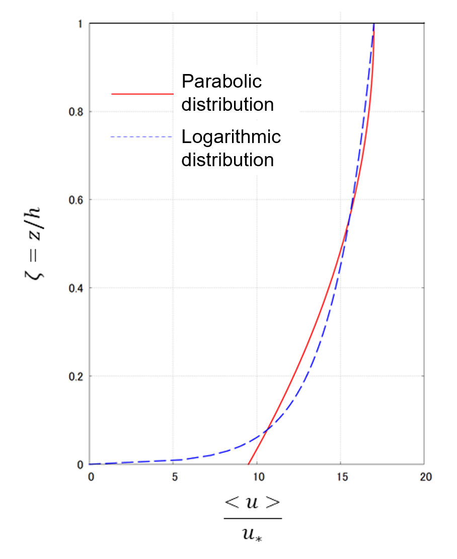
Figure 8 : Comparison of the logarithmic law and parabolic distribution

Karman-Prandtl’s equation for the near-wall turbulent flow velocity ([Ref:31])

Karman-Prandtl proposed the following equation as the flow velocity equation for near-wall turbulence ([Ref:31] ).

(61)\[\cfrac{u}{u_\ast}= A + \cfrac{1}{\kappa}\ln \cfrac{z}{k_s} =A +5.75\log \cfrac{z}{k_s}\]

Where, \(u\) is the flow velocity, \(\kappa\) is Karman’s constant, \(A\) is an experimental constant, \(u_\ast\) is the friction velocity, \(z\) is the distance from the wall, and \(k_s\) is the roughness height.

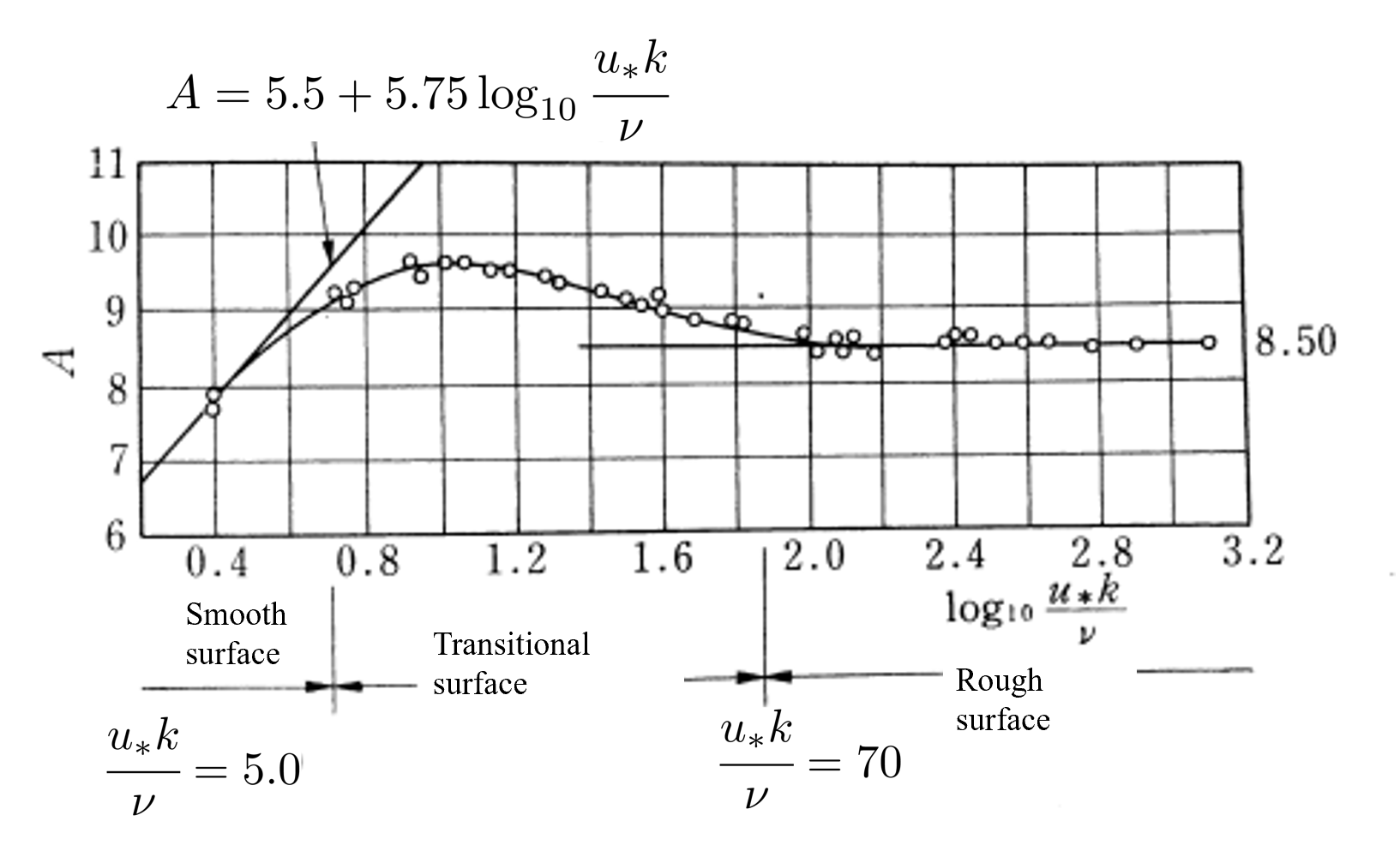
Figure 9 : Calculation of constant \(A\) for the velocity distribution equation

From the experimental results of Nikuradse shown in Figure 9, the constant \(A=8.5\) is obtained for rough surfaces, and from this, Equation (61) derives…

(62)\[ \cfrac{u}{u_\ast}= 8.5 + \cfrac{1}{\kappa}\ln \cfrac{z}{k_s}\]

Assuming that this is equal to the theoretical equation of the logarithmic law, Equation (41), we obtain the following.

(63)\[\cfrac{u}{u_\ast}=8.5 + \cfrac{1}{\kappa}\ln \cfrac{z}{k_s} = \cfrac{1}{\kappa}\ln \cfrac{z}{z_0}\]

And assuming that \(\kappa=0.4\), we have…

(64)\[k_s=29.96 z_0 \approx 30z_0\]

Roughness of a flat riverbed

Here we discuss the roughness of a flat riverbed (without the influence of riverbed waves). An exponential approximation of the mean velocity equation (Equation (47)) based on the logarithmic law is easier to deal with.

(65)\[\cfrac{<u>}{u_\ast} = 6+5.75 \log{\cfrac{h}{k_s}} \approx 7.66\left(\displaystyle{{h}\over{k_s}}\right)^{1/6}\]

This is illustrated in Figure 10, which shows a close approximation.

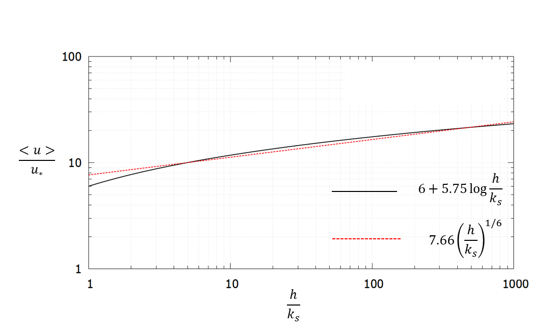
Figure 10 : Exponential approximation of the logarithmic velocity equation

Expression with the Manning’s roughness coefficient

Regarding the relationship between Manning’s law and the roughness, assuming that \(n_m\) is Manning’s roughness coefficient, and because…

(66)\[<u>=\cfrac{1}{n_m} h^{2/3} I_e^{1/2} = 7.66 \left(\cfrac{h}{k_s}\right)^{\cfrac{1}{6}} \sqrt{g h I_e}\]

we have…

(67)\[n_m = \cfrac{1}{7.66} \cfrac{{k_s}^{1/6}}{g^{1/2}}\]

or,

(68)\[k_s = (7.66 n_m g^{1/6})^6 = 2.02 \times 10^5 g {n_m}^6\]

Manning’s law uses [meter, sec] for the units of measurement, in principle. By setting \(g\) as 9.8 (m/s \(^2\)), we have…

(69)\[n_m=0.0415 {k_s}^{1/6} \mbox{or} k_s=1.98 \times 10^6 {n_m}^6\]

For a flat riverbed, using the equivalent roughness height \(k_s=2d\) (\(d\) is the grain size of the bed material), we have…

(70)\[n_m=0.015d^{1/6}\]

Where, unit of \(d\) is [mm].

Regarding the relationship between the roughness and the coefficients of resistance and flow velocity

When the roughness of a flat riverbed is expressed with the grain size of the riverbed material by using the coefficients of resistance, such as the velocity coefficient, \(\varphi\) and the friction coefficient, \(C_f\), then that roughness is expressed as follows.

(71)\[\cfrac{<u>}{u_\ast} = \varphi = \cfrac{1}{\sqrt{C_f}}\]

Consequently, we have…

(72)\[\begin{split}C_f = \cfrac{1}{\varphi^2} = \cfrac{{u_\ast}^2}{<u>^2} \\ \varphi = \cfrac{h^{1/6}}{n_m \sqrt{g}} \\ C_f = \cfrac{g {n_m}^2}{h^{1/3}}\end{split}\]

The above is an example expression.