4. 1D unsteady flow with constant width

4.1. Basic formulas

The equation of motion and the equation for continuity for unsteady flow in a channel with a constant width and a triangular cross section are…

(4.1)\[{{\partial h}\over{\partial t}} +{{\partial (uh)}\over{\partial x}} = 0\]

(4.2)\[{{\partial (uh)}\over{\partial t}} +{{\partial (u^2 h)}\over{\partial x}} = -gh{{\partial H}\over{\partial x}} + \cfrac{\partial}{\partial x} \left\{ \varepsilon \cfrac{\partial (uh)}{\partial x} \right\} -{{\tau_x}\over{\rho}}\]

Where, \(t\) is the time, \(x\) is the distance in the flow direction, \(h\) is the water depth, \(u\) is the flow velocity, \(g\) is the gravitational acceleration, \(H\) is the water level, \((=z_b+h)\), \(z_b\) is the riverbed elevation, \(\varepsilon\) is the eddy viscosity coefficient, \(\tau_x\) is the riverbed shear force, and \(\rho\) is the water density.

The left side of Equation (4.2) is expressed in a form called the “conservation form”. This makes the equation applicable to a water surface with a discontinuous profile. When the water surface has a continuous profile, this means that when and \(\displaystyle{{\partial h}\over{\partial x}}\) and \(\displaystyle{{\partial u}\over{\partial x}}\) are present, the left side of Equation (4.2) is as follows.

(4.3)\[u{{\partial h}\over{\partial t}} +h{{\partial u}\over{\partial t}} + u{{\partial(uh)}\over{\partial x}} +uh{{\partial u}\over{\partial x}}\]

It is possible to develop the equation. Using the equation of continuity, Equation (4.1), Equation (4.2) can be converted into the following equation. Note that the diffusion term is an approximation.

(4.4)\[{{\partial u}\over{\partial t}} +u{{\partial u}\over{\partial x}} = -g{{\partial H}\over{\partial x}} + \varepsilon {{\partial^2 u}\over{\partial x^2}}-{{\tau_x}\over{\rho h}}\]

The following explanations use this non-conservation form of Equation (4.4) for the equation of motion. As a basis, a non-conservation form of the equation of motion cannot deal with discontinuous flow. However, it is known that the CIP method can deal with such a flow to some extent. This is probably because the 3D interpolation function deployed by the CIP method is able to address sudden points of change in the function to some extent.

4.2. Preparation for applying the CIP method (the split method)

To further simplify the discussion, we consider the case where the riverbed shear force (friction) is negligible and the viscosity is also negligible. The basic formulas are…

(4.5)\[{{\partial h}\over{\partial t}} +{{\partial (uh)}\over{\partial x}} = 0\]

(4.6)\[{{\partial u}\over{\partial t}} +u{{\partial u}\over{\partial x}} = -g{{\partial H}\over{\partial x}}\]

As you can see from the equations, the main difference is that, as in Equation (3.29), before there was only one unknown variable, \(f\), but now there are two unknown variables, \(h\) and \(u\). You can understand the calculation procedure intuitively from the time differential term. We calculate \(h\) with Equation (4.5), and \(u\) with Equation (4.6). A split method is applied to Equation (4.6) as it is applied to Equation (3.29). Therefore, the split is as follows.

(4.7)\[{{\partial u}\over{\partial t}} = -g \displaystyle{\left( {{\partial h}\over{\partial x}} + {{\partial z_b}\over{\partial x}} \right) }\]

(4.8)\[{{\partial u}\over{\partial t}}+u{{\partial u}\over{\partial x}} = 0\]

Note that the relationship of \(H=h+z_b\) is applied. To calculate \(u^n \rightarrow u^{n+1}\) by using Equation (4.6), place \(\widetilde{u}\) in the middle, calculate \(u^n \rightarrow \widetilde{u}\) with Equation (4.7), and calculate \(\widetilde{u} \rightarrow u^{n+1}\) with Equation (4.8). Equation (4.7) includes \(h\). Therefore, when calculating Equation (4.7), Equation (4.5) must be satisfied at the same time. Therefore, let us express it as \(h^n \rightarrow \widetilde{h}\). However, Equation (4.8) does not include \(h\). Therefore, it is impossible to relate it to Equation (4.5). \(\widetilde{h}\) is the simultaneous solution of Equation (4.5) and Equation (4.7) and it is used “as is” for \(h^{n+1}\), as follows.

(4.9)\[h^{n+1}=\widetilde{h}\]

The above is summarized in the table below.

Table 4.1 Split method for 1D unsteady flow

Phase name	Updating \(u\) and \(h\)	Equation used
[A] non-advection phase	\(u^n \rightarrow \widetilde{u}, h^n \rightarrow \widetilde{h}\)	Equations (4.7) and (4.5)
[B] advection phase	\(\widetilde{u} \rightarrow u^{n+1}, \widetilde{h} \rightarrow h^{n+1}\)	Equations (4.8) and (4.9)

4.3. The non-advection phase

First, we calculate \(u^n \rightarrow \widetilde{u}\) with Equation (4.7). At the same time, we perform \(h^n \rightarrow \widetilde{h}\) with Equation (4.5). Then, Equation (4.7) is expressed as follows.

(4.10)\[{{\widetilde{u}-u^n}\over{\Delta t}} = -g \displaystyle{ \left( {{\partial \widetilde{h}}\over{\partial x}} + {{\partial z_b}\over{\partial x}} \right) }\]

Therefore, we obtain…

(4.11)\[\widetilde{u}= u^n - g \Delta t {{\partial \widetilde{h}}\over{\partial x}} - g \Delta t {{\partial z_b}\over{\partial x}}\]

Meanwhile, because we obtain \(h^n \rightarrow \widetilde{h}\) with Equation (4.5), the following equation should be satisfied.

(4.12)\[{{\widetilde{h}-h^n}\over{\Delta t}} + {{\partial}\over{\partial x}} (\widetilde{u} \widetilde{h} ) =0\]

Therefore, we need to obtain \(\widetilde{h}\) and \(\widetilde{u}\), the simultaneous solutions to Equation (4.11) and Equation (4.12).

In general, when the CIP method is applied to the calculation of a fluid, we use a staggered grid in which the calculation points of \(u\) and \(h\) are alternately arranged. Here, let us deploy the arrangement of calculation points shown in Figure 4.1 .

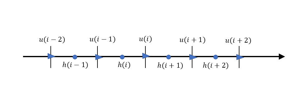
Figure 4.1 : Staggered grids

Taking into account this arrangement of calculation points, the difference expression of Equation (4.11) is…

(4.13)\[\widetilde{u}(i) = u^n(i)-g\Delta t {{\widetilde{h}(i+1) - \widetilde{h}(i)}\over{\Delta x}} -g\Delta t {{z_b(i+1) - z_b(i)}\over{\Delta x}}\]

(Here, we assume that the calculation points of \(z_b\) are the same as those of \(h\).) To substitute this for the second term on the left side of Equation (4.12), we introduce the unit width discharge, \(q\), that satisfies…

(4.14)\[\widetilde{q}=\widetilde{u} \widetilde{h}\]

(The calculation points of \(q\) are the same as those of \(u\).) Considering the arrangement of grid points, we use the following equation,

(4.15)\[\widetilde{q}(i)= \widetilde{u}(i) {{\widetilde{h}(i+1)+\widetilde{h}(i)}\over{2}}\]

in addition to the following difference equation of Equation (4.12) that adopted \(q\).

(4.16)\[\widetilde{h}(i) = h^n(i) - \left[ \widetilde{q}(i)-\widetilde{q}(i-1) \right] {{\Delta t}\over{\Delta x}}\]

Then, we obtain \(\widetilde{h}\). However, \(\widetilde{q}\) in the right side of Equation (4.16) also contain \(\widetilde{h}\) in implicit form. As shown in Figure 4.2, we need to repeat the calculations.

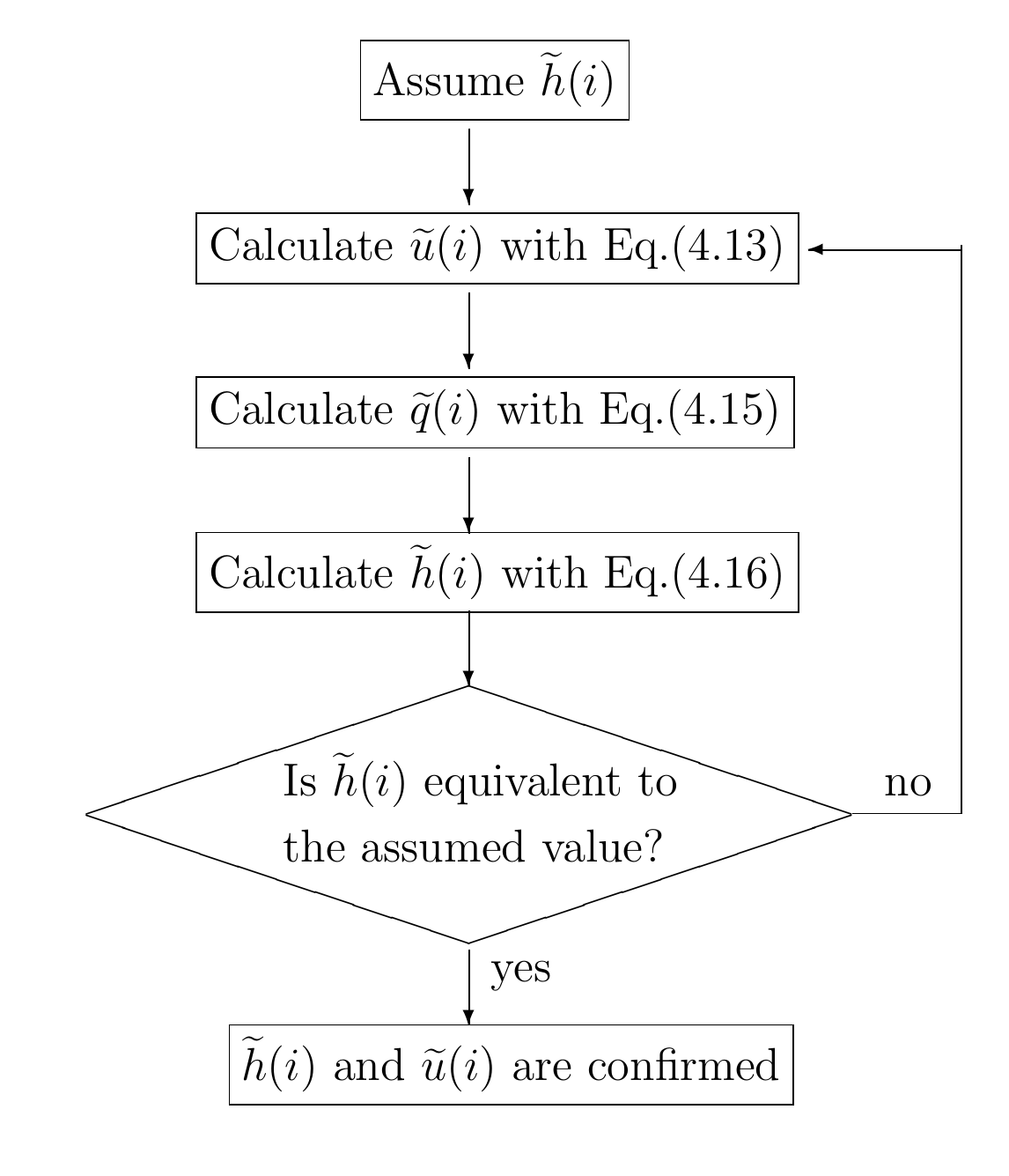
Figure 4.2 : The flow of calculation of \(\widetilde{h}(i)\) and \(\widetilde{u}(i)\) in the non-advection phase

These repetitions of calculation give us \(\widetilde{h}(i)\) and \(\widetilde{u}(i)\). They are the calculation results for the non-advection phase.

Once, \(\widetilde{u}(i)\) for the non-advection phase is obtained, then \(\displaystyle{\widetilde{{\partial u}\over{\partial x}}}\) for the non-advection phase needs to be obtained. It can be obtained from the following equation, which is obtained by replacing \(f\) with \(u\) in Equation (3.38).

(4.17)\[\widetilde{{\partial u}\over{\partial x}}(i)= {{\partial u}\over{\partial x}}^n(i)+{{1}\over{2\Delta x}} \left[ \widetilde{u}(i+1)-u^n(i+1)-\widetilde{u}(i-1)+u^n(i-1) \right]\]

4.4. The advection phase

In the advection phase, the CIP method can be applied directly to Equation (4.8). By replacing \(f\) with \(u\) in Equation (3.39), the following equation gives the solution.

(4.18)\[{u(i)}^{n+1}=U(X)= \left[(aX+b)X+ \widetilde{{\partial u}\over{\partial x}}(i) \right] X +\widetilde{u}(i)\]

Where, \(\widetilde{u}(i)\) and \(\displaystyle{\widetilde{{\partial u}\over{\partial x}}(i)}\) are \(u\) and the spatial differentiation amounts of \(u\) in the non-advection phase, respectively. \(\displaystyle{\widetilde{{\partial u}\over{\partial x}}(i)}\) They are obtained from equations (4.13) and (4.17), respectively. Also, \(a\) and \(b\) are given by Equation (3.27) in the previous chapter, by replacing \(f\) with \(u\).

Therefore, using \(U(X)\), \(u\) in the advection phase is…

(4.19)\[u(i)^{n+1}= U(X)\]

Similarly, the spatial differentiation amount of \(u\) in the advection phase can be obtained from Equation (3.45) and Equation (3.47) by substituting \(f\) with \(u\) as follows.

(4.20)\[\widehat{{\partial u}\over{\partial x}}(i) = 3aX^2 + 2bX + \widetilde{{\partial u}\over{\partial x}}(i)\]

and

(4.21)\[{{\partial u}\over{\partial x}}^{n+1}(i) = \widehat{{\partial u}\over{\partial x}}(i) -{{u(i+1)-u(i-1))}\over{2\Delta x}}\widehat{{\partial u}\over{\partial x}}(i) \Delta t\]

4.5. Boundary conditions

To use the CIP method for this calculation method, in addition to needing the boundary conditions of \(u\) and \(h\), we also need the boundary conditions of \(\displaystyle{{\partial u}\over{\partial x}}\). Physical boundary conditions are required that are in line with the phenomenon that is subject to the calculation. The simplest condition is that for all variables, applying below.

(4.22)\[{{\partial}\over{\partial x}} =0\]

This is a free boundary condition. The water level (water depth) must be selected according to the calculation conditions. The details are omitted, but the water level (water depth) boundary conditions at the downstream end can be given for ordinary flow, and those at the upstream end can be given for jet flow. Note that, of course, the boundary conditions must be applied to both the non-advection phase and the advection phase.

4.6. Summary

The flowchart below summarizes the above calculations for the 1D flow with free water surface.

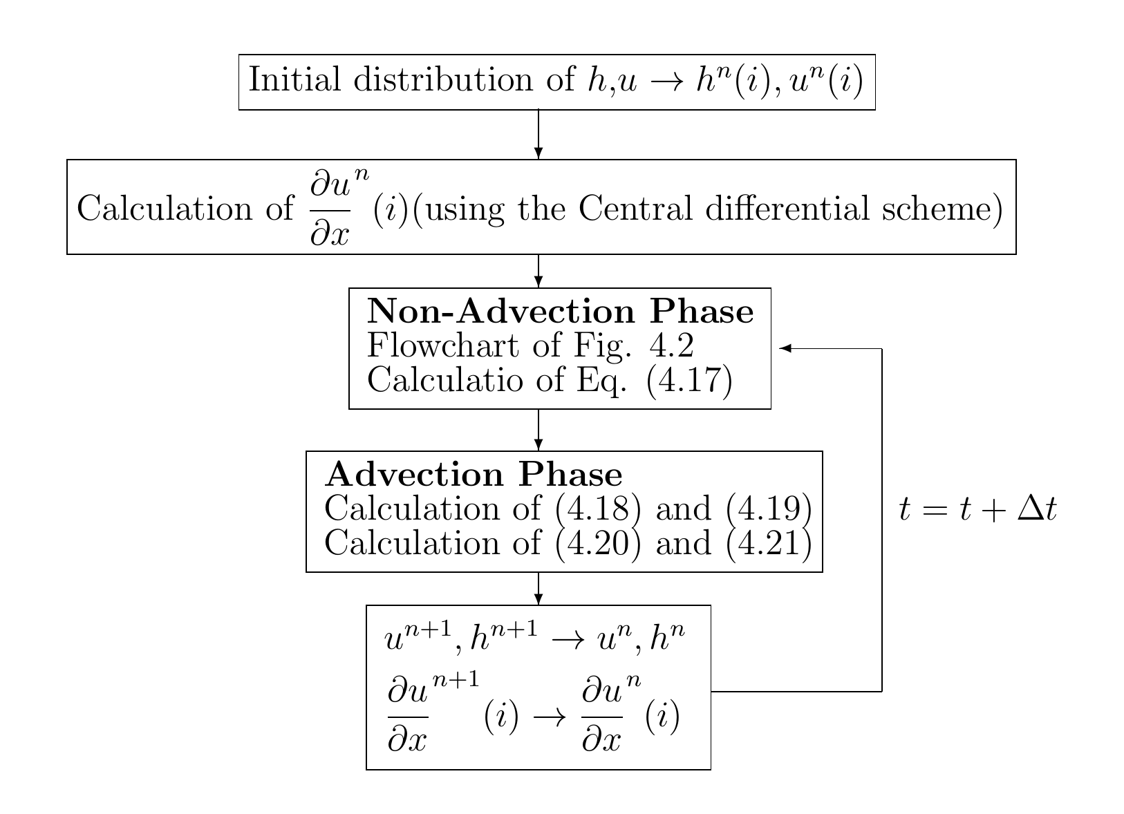
Figure 4.3 : Flow chart for the 1D flow calculation with free water surface

4.7. The Python code

An example of code for the above 1D unsteady flow calculation is below.

https://github.com/YasuShimizu/1D-Free-Water-Surface

Files in this GitHub folder with the extension “py” are the calculation files. Of these, “main.py” file is the main body of the calculation code. Of which, the following part can be used for water surface profile calculations under different conditions　by　sequentially activating the part of the code with the “yml” file name commented out.

with open('config.yml','r', encoding='utf-8') as yml:
#with open('config_jump.yml','r', encoding='utf-8') as yml:   # hydraulic jump
#with open('config_trans.yml','r', encoding='utf-8') as yml:  # transitional flow
#with open('config_back_water.yml','r', encoding='utf-8') as yml:   # back water
#with open('config_drop_down.yml','r', encoding='utf-8') as yml:   # drawdown
#with open('config_bump.yml','r', encoding='utf-8') as yml:   # flow in a channel with a bump
    config = yaml.load(yml)

The yml file describes the calculation conditions and is included on the above GitHub site. As an example, [config_trans.yml] is shown below. Calculations can be carried out while the conditions are changed by appropriately modifying the items in the comments. For simplicity, the explanation of the calculation method assumes that friction is negligible. In the code, however, a friction term is added to the equations of motion. By setting the coefficient of roughness to zero in the “yml” file, calculations ignoring friction can be performed.

xl : 200 # channel length (m)
nx: 51  # no. of grids in the x-direction
j_channel: 2 # condition of the channel (1=constant gradient, 2=gradient changes)
# when j_channel=1
slope: 0.002 # entire gradient
# when j_channel=2
x_slope : 130 # gradient changing point
slope1 : 0.001 # upstream gradient
slope2 : 0.01 # downstream gradient
xb1 : 4 # distance from the upstream end to the bump starting point (m)
xb2 : 5 # distance from the upstream end to the bump crest (m)
xb3 : 6 # distance from the upstream end to the bump ending point (m)
dbed : 0.00 # bump height (m)
qp : 1 # unit width discharge (m**2/2)
g : 9.8 # gravitational acceleration
snm : 0.025 # coefficient of roughness
alh : 0.6 # relaxation factor for water level calculation
lmax : 50 # max. replication number of water level calculation
errmax : 0.0001 # truncation error
hmin : 0.01 # min. water depth (m)
j_upstm : 2 # condition of upstream end (1=wall, 2=free, 3=fixed value)
j_dwstm : 3 # condition of the downstream end
alpha_up: 1.0 # water depth at the upstream end (ratio over the neutral depth)
alpha_dw: 1.0 # water depth at the downstream end (ratio over the neutral depth)

etime : 400 # calculation end time (sec)
dt : 0.05 # calculation time step (sec)
tuk : 10 # output interval

Regarding xb1, xb2, xb3 and dbed in [config_trans.yml], they are defined as shown in the following figure.

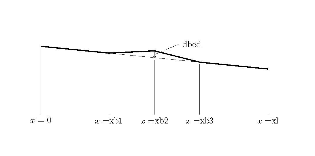
Figure 4.4 : Parameter for setting the riverbed bump

4.8. Calculation example

4.8.1. Back water

Examples of calculation results using [config_back_water.yml] are below. The calculation results are from the top, longitudinal profiles of the water level (Water), the bed morphology (Bed), the velocity (Velocity), the unit width discharge (Discharge), and the Froude number (Fr). Equation (4.23) gives the neutral depth, \(h_0\), and the critical water depth, \(h_c\). They are also shown with the longitudinal profiles of water level.

(4.23)\[h_0=\left(\cfrac{q n}{\sqrt{i}}\right)^{3/5}, \ \ h_c=\left(\cfrac{q^2}{g}\right)^{1/3}\]

Figure 4.5 : Calculating an example of back water

The calculations of Figure 4.5 show how the effect of the water level being raised to 20% deeper than the isobath at the downstream end is transmitted upstream.

4.8.2. Drawdown

Figure 4.6 shows the the calculation results using [config_drop_down.yml]. In this example, we calculate the conditions of the drawdown whose boundary condition is the water depth at the downstream end being kept at 70% of the neutral depth.

Figure 4.6 : Examples of drawdown calculation

4.8.3. Hydraulic jump

Figure 4.7 shows the calculation results using [config_jump.yml]. In this example, the hydraulic jumps are calculated for a channel with a steep gradient at the upper reaches and a gentle gradient at the lower reaches.

Figure 4.7 : Examples of hydraulic jump calculation

4.8.4. Transitional flow

Figure 4.8 shows the calculation results using [config_trans.yml]. In this example, the transition from ordinary flow to jet flow is calculated in a channel with a gentle gradient at the upstream end and a steep gradient at the downstream end.

Figure 4.8 : Examples of transitional flow calculation

4.8.5. Flow in a channel with a bump at the channel center

Figure 4.9 shows the calculation results using [config_bump.yml]. In this example, the flow is calculated for a channel with a bump at the longitudinal midpoint of the channel. Because this example is for ordinary flow, the water level is calculated to be less over the bump than elsewhere. (You studied this phenomena in your hydraulics class. Do you remember?)

Figure 4.9 : Calculation examples for flow in a channel with a bump at the longitudinal midpoint of the channel.