7. 2-dimensional unsteady flow with free water surface

This chapter describes a method for calculating 2D unsteady flow with a free water surface. The flow field dealt with here does not take into account the distribution of velocities in the depth direction nor the velocity components in the vertical direction. The depth scale is considerably small relative to the planar scale, i.e., the flow is relatively shallow. It is also called 2D shallow flow. The basic formulas of 2D shallow flow consist of the following equation of continuity…

(7.1)\[\frac{\partial h}{\partial t}+\frac{\partial (uh)}{\partial x}+ \frac{\partial (vh)}{\partial y}=0\]

…and of the following equations of motion.

(7.2)\[\frac{\partial u}{\partial t}+u \frac{\partial u}{\partial x}+ v \frac{\partial u}{\partial y}= -g \frac{\partial H}{\partial x} -\frac{\tau_x}{\rho h}+ \frac{\partial}{\partial x} (\nu_t \frac{\partial u}{\partial x})+ \frac{\partial}{\partial y} (\nu_t \frac{\partial u}{\partial y})\]

(7.3)\[\frac{\partial v}{\partial t}+u \frac{\partial v}{\partial x}+ v \frac{\partial v}{\partial y}= -g \frac{\partial H}{\partial y} -\frac{\tau_y}{\rho h}+ \frac{\partial}{\partial x} (\nu_t \frac{\partial v}{\partial x})+ \frac{\partial}{\partial y} (\nu_t \frac{\partial v}{\partial y})\]

Where, \(x, y\) are the plane coordinate axes that are perpendicular to each other, \(t\) is time, \(u, v\) are depth-averaged velocity in the \(x, y\) directions, \(h\) is the water depth, \(H\) is the water level, \(g\) is the gravitational acceleration, \(\tau_x, \tau_y\) are the bed shear force in the directions of \(x, y\), \(\rho\) is the density of water and \(\nu_t\) is the turbulent eddy viscosity.

Using the Manning formula for the law of resistance, the bed shear force is expressed as follows.

(7.4)\[\frac{\tau_x}{\rho h}= \frac{gn^2}{h^{4/3}} u\sqrt{u^2+v^2}, \ \ \ \frac{\tau_y}{\rho h}= \frac{gn^2}{h^{4/3}} v\sqrt{u^2+v^2}\]

Where, \(n\) is the Manning’s roughness coefficient.　　Regarding the deliberation of Equation (7.4), refer to Expressions of riverbed shear force in Appendix. Deploying a zero-equation model, the turbulent eddy viscosity is expressed as follows.

(7.5)\[\nu_t = \frac{\kappa}{6} u_\ast h\]

Where, \(u_\ast\) is the friction velocity,

(7.6)\[u_\ast=\sqrt{ghI_f}\]

\(I_f\) is the gradient of friction velocity as expressed by the following equation.

(7.7)\[I_f=\frac{n^2 (u^2+v^2)}{h^{4/3}}\]

7.1. Basic formulas and the application of the split method

For the calculation of 2D unsteady flow with a free-surface, Equation (7.1) is used to calculate the water depth, \(h\), Equation (7.2), the equation of motion in the \(x\) direction, is used to calculate the flow velocity, \(u\), in the \(x\) direction; and Equation (7.2), the equation of motion in the \(y\) direction, is used to calculate the flow velocity, \(v\), in the \(y\) direction. When the riverbed elevation, \(\eta\), is given, the water level, \(H=\eta+h\) is \(H=\eta+h\). \(H=\eta+h\) has a univalent correspondence with \(h\). Then, instead of \(h\), we can treat \(H\) as an unknown value.

As performed for the case of 1D, the split method is applied to Equation (7.2) and Equation (7.3). Because their forms are almost the same, an explanation is given only for Equation (7.2), here. Now, we rewrite Equation (7.2) as follows by applying the relationship of \(H=\eta+h\). For your confirmation, these equations are shown again.

(7.8)\[{{\partial u}\over{\partial t}}+u {{\partial u}\over{\partial x}}+v{{\partial u}\over{\partial y}} = -g \left( {{\partial h}\over{\partial x}}+{{\partial \eta}\over{\partial x}} \right) -{{g n_m^2 u\sqrt{u^2+v^2}}\over{h^{4/3}}} +\nu_t \left[ {{\partial^2 u}\over{\partial x^2}} + {{\partial^2 u }\over{\partial y^2}} \right]\]

This equation has an advection term. Thus, the equation is split into three equations. Each includes one part related to the advection term, one to the pressure and friction terms, and one to the diffusion term.

(7.9)\[{{\partial u}\over{\partial t}} = -g \displaystyle{\left( {{\partial h}\over{\partial x}} + {{\partial \eta}\over{\partial x}} \right) } -{{g n_m^2 u\sqrt{u^2+v^2}}\over{h^{4/3}}}\]

(7.10)\[{{\partial u}\over{\partial t}} = \nu_t \displaystyle{\left[ {{\partial^2 u }\over{\partial x^2}} +{{\partial^2 u}\over{\partial y^2}} \right] }\]

(7.11)\[{{\partial u}\over{\partial t}}+ u{{\partial u}\over{\partial x}} +v{{\partial u}\over{\partial y}} = 0\]

Now, \(n\) is a time step. Instead of calculating \(u^n \rightarrow u^{n+1}\) with Equation (7.8), assuming \(\overline{u}\) and \(\widetilde{u}\) are in the middle, let us calculate \(u^n \rightarrow \overline{u}\) with Equation (7.9), \(\overline{u} \rightarrow \widetilde{u}\) with Equation (7.10), and \(\widetilde{u} \rightarrow u^{n+1}\) with Equation (7.11). Because Equation (7.9) includes \(h\), the solutions should also satisfy the equation of continuity, Equation (7.1). Therefore, let us express it as \(h^n \rightarrow \overline{h}\). On the other hand, because Equation (7.10) and Equation (7.11) do not include \(h\), we use \(\overline{h}\) for \(h^{n+1}\) as follows.

(7.12)\[h^{n+1} = \overline{h}\]

For \(v\), we perform exactly the same procedure as above. The equation of motion for \(v\) is also split, as follows.

(7.13)\[{{\partial v}\over{\partial t}} = -g \displaystyle{\left( {{\partial h}\over{\partial y}} + {{\partial \eta}\over{\partial y}} \right) } -{{g n_m^2 v\sqrt{u^2+v^2}}\over{h^{4/3}}}\]

(7.14)\[{{\partial v}\over{\partial t}} = \nu_t \displaystyle{\left[ {{\partial^2 v }\over{\partial x^2}} +{{\partial^2 v}\over{\partial y^2}} \right] }\]

(7.15)\[\cfrac{\partial v}{\partial t}+u\cfrac{\partial v}{\partial x} +v\cfrac{\partial v}{\partial y} = 0\]

The above is summarized as follows.

Table 7.1 Split method for 2D flow

Phase name	Procedure			Equations used
Non-advection phase I	\(u^n \rightarrow \overline{u}\)	\(v^n \rightarrow \overline{v}\)	\(h^n \rightarrow \overline{h} \rightarrow h^{n+1}\)	Eqs. (7.9), (7.13), (7.1), and (7.12)
Non-advection phase II	\(\overline{u} \rightarrow \widetilde{u}\)	\(\overline{v} \rightarrow \widetilde{v}\)		Eqs. (7.10) and (7.14)
Advection phase	\(\widetilde{u} \rightarrow u^{n+1}\)	\(\widetilde{v} \rightarrow v^{n+1}\)		Eqs. (7.11) and (7.15)

Now, we are ready to apply the CIP method.

7.2. The non-advection phase I

We calculate \(u^n \rightarrow \overline{u}\) with Equation (7.9), and \(v^n \rightarrow \overline{n}\) with Equation (7.13). Now, let us rewrite equations (7.9) and (7.13) as follows.

(7.16)\[{{\overline{u}-u^n}\over{\Delta t}} = -g \displaystyle{ \left( {{\partial \overline{h}}\over{\partial x}} + {{\partial \eta}\over{\partial x}} \right) } -{{g n_m^2 \overline{u} \sqrt{\overline{u}^2 +\overline{v}^2}} \over{\overline{h}^{4/3}}}\]

(7.17)\[{{\overline{v}-v^n}\over{\Delta t}} = -g \displaystyle{ \left( {{\partial \overline{h}}\over{\partial y}} + {{\partial \eta}\over{\partial y}} \right) } -{{g n_m^2 \overline{v} \sqrt{\overline{u}^2 +\overline{v}^2}} \over{\overline{h}^{4/3}}}\]

Therefore, we have…

(7.18)\[\overline{u}= u^n - g \Delta t {{\partial \overline{h}}\over{\partial x}} - g \Delta t {{\partial \eta}\over{\partial x}} - g \Delta t {{n_m^2 \overline{u}\sqrt{\overline{u}^2 +\overline{v}^2}} \over{\overline{h}^{4/3}}}\]

(7.19)\[\overline{v}= v^n - g \Delta t {{\partial \overline{h}}\over{\partial y}} - g \Delta t {{\partial \eta}\over{\partial y}} - g \Delta t {{n_m^2 \overline{v}\sqrt{\overline{u}^2 +\overline{v}^2}} \over{\overline{h}^{4/3}}}\]

Meanwhile, because we obtain \(h^n \rightarrow \overline{h}\)　by using Equation (7.1), the following equation should be satisfied.

(7.20)\[{{\overline{h}-h^n}\over{\Delta t}} + {{\partial}\over{\partial x}} (\overline{u} \overline{h}) + {{\partial}\over{\partial y}} (\overline{v} \overline{h})=0\]

Therefore, we need to solve the simultaneous equations (7.18) \(\sim\) (7.20) so as to obtain \(\overline{h}\), \(\overline{u}\) and \(\overline{v}\).

In general, when the CIP method is applied to the calculation of a fluid, we use a staggered grid in which calculation points of \(u\), \(v\) and \(h\) are alternately placed. Here, let us deploy the setting of calculation points shown in Figure 7.1.

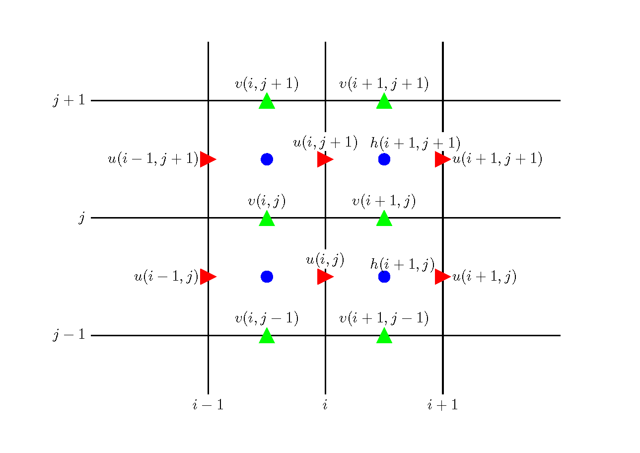
Figure 7.1 : Arrangement of calculation grids

Taking into account of the arrangement of calculation points in Figure 7.1, the difference expression of Equation (7.18) is as follows.

(7.21)\[\begin{split}\overline{u}(i,j) = & u^n(i,j)-g\Delta t {{\overline{h}(i+1,j) - \overline{h}(i,j)}\over{\Delta x}} -g\Delta t {{\eta(i+1,j) - \eta(i,j)}\over{\Delta x}} \\ & - g \Delta t {{n_m^2 \overline{u}(i,j) \sqrt{\overline{u}(i,j)^2+\overline{v_{up}}^2} }\over{\overline{h_{up}}^{4/3}}}\end{split}\]

Where, subscript, \(_{up}\), means it is a value at the calculation point of \(u\). The arrangement of calculation points in Figure 7.1 gives…

(7.22)\[\overline{v_{up}}={{\overline{v}(i,j)+\overline{v}(i,j-1) +\overline{v}(i+1,j)+\overline{v}(i+1,j-1)}\over 4}\]

(7.23)\[\overline{h_{up}}={{\overline{h}(i,j)+\overline{h}(i+1,j)}\over 2}\]

Similarly, the difference expression of Equation (7.19) is…

(7.24)\[\begin{split}\overline{v}(i,j) = & v^n(i,j)-g\Delta t {{\overline{h}(i,j+1) - \overline{h}(i,j)}\over{\Delta y}} -g\Delta t {{\eta(i,j+1) - \eta(i,j)}\over{\Delta y}} \\ & - g \Delta t {{n_m^2 \overline{v}(i,j) \sqrt{\overline{u_{vp}}^2+\overline{v}(i,j)^2} }\over{\overline{h_{vp}}^{4/3}}}\end{split}\]

The subscript \(_{vp}\) indicates that it is the value of \(u\) at the calculation point, and we have…

(7.25)\[\overline{u_{vp}}={{\overline{u}(i,j)+\overline{u}(i-1,j) +\overline{u}(i,j+1)+\overline{u}(i-1,j+1)}\over 4}\]

(7.26)\[\overline{h_{vp}}={{\overline{h}(i,j)+\overline{h}(i,j+1)}\over 2}\]

To substitute Equation (7.21) and Equation (7.24) for the second and third terms on the left side of Equation (7.20), we make the following definitions.

(7.27)\[\overline{q_u}=\overline{u} \overline{h}, \; \; \; \overline{q_v}=\overline{v} \overline{h}\]

In consideration of the arrangement of grid points (the calculation points of \(q_u`n and :math:`q_v\) are assumed to be the same as \(u\) and \(v\), respectively). Now, we have…

(7.28)\[\overline{q_x}(i,j)= \overline{u}(i,j) {{\overline{h}(i+1,j)+\overline{h}(i,j)}\over{2}}\]

(7.29)\[\overline{q_y}(i,j)= \overline{v}(i,j) {{\overline{h}(i,j+1)+\overline{h}(i,j)}\over{2}}\]

Together with the following difference expression of Equation (7.20) that uses \(q_x\) and \(q_y\)…

(7.30)\[\overline{h}(i) =h^n(i,j) + \left[ {{\overline{q_x}(i,j)-\overline{q_x}(i-1,j)}\over{\Delta x}} +{{\overline{q_y}(i,j)-\overline{q_y}(i,j-1)}\over{\Delta y}} \right]\Delta t\]

…we can obtain \(\overline{h}\). However, \(\overline{q_x}\) and \(\overline{q_y}\) on the right side of Equation (7.30) also contain \(\overline{h}\) in implicit form, which require calculation repetitions to solve the equation. This procedure is shown in Figure 7.2.

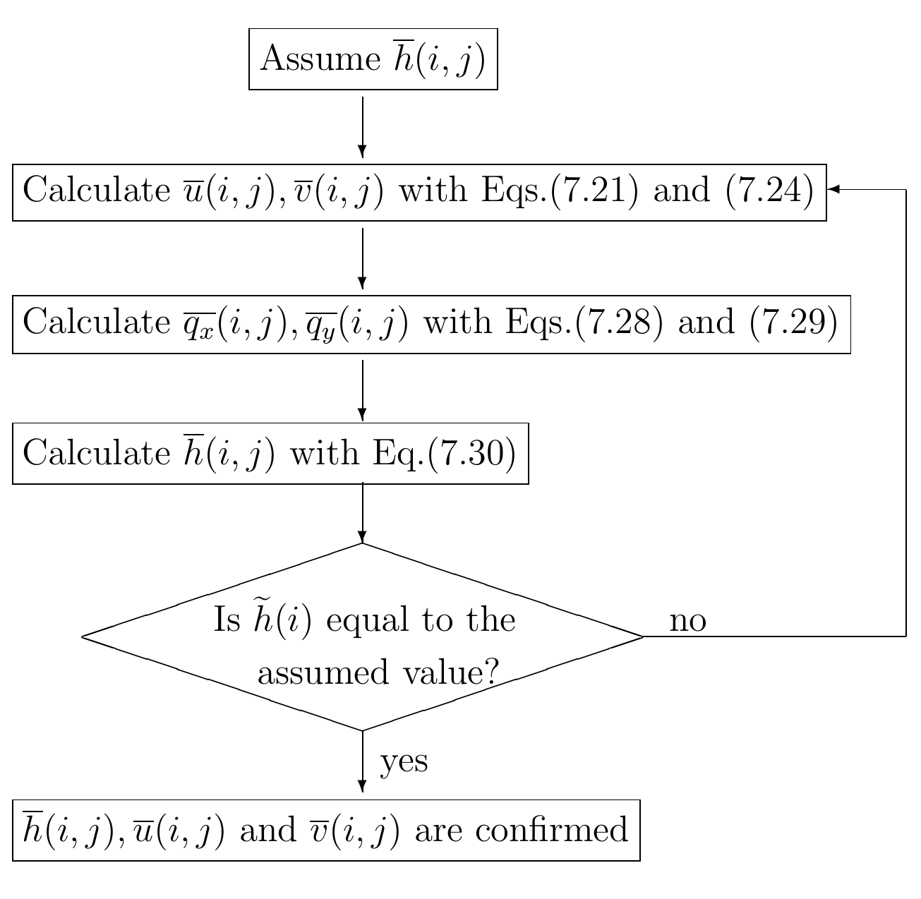
Figure 7.2 : Flow of calculation procedure for \(\overline{h}(i,j)\), \(\overline{u}(i,j)\) and \(\overline{v}(i,j)\) in non-advection phase I

The calculation repetitions give \(\overline{h}(i)\), \(\overline{u}(i,j)\) and \(\widetilde{v}(i,j)\). They are calculation results for non-advection phase I.

When \(\overline{u}(i,j)\) and \(\overline{u}(i,j)\) in non-advection phase I are obtained, \(\displaystyle{{\partial u}\over{\partial x}}\) , \(\displaystyle{{\partial u}\over{\partial y}}\) , \(\displaystyle{{\partial v}\over{\partial x}}\) and \(\displaystyle{{\partial v}\over{\partial y}}\) i.e., \(\overline{\displaystyle{{\partial u}\over{\partial x}}}\), \(\overline{\displaystyle{{\partial u}\over{\partial y}}}\) , \(\overline{\displaystyle{{\partial v}\over{\partial x}}}\) and \(\overline{\displaystyle{{\partial v}\over{\partial y}}}\) for non-advection phase I need to be calculated. As for the 1D case, they can be calculated by using the following equations.

(7.31)\[\overline{{\partial u}\over{\partial x}}(i,j)= {{\partial u}\over{\partial x}}^n(i,j) +{{1}\over{2\Delta t}} \left[ \overline{u}(i+1,j)-u^n(i+1,j)-\overline{u}(i-1,j)+u^n(i-1,j) \right]\]

(7.32)\[\overline{{\partial u}\over{\partial y}}(i,j)= {{\partial u}\over{\partial y}}^n(i,j) +{{1}\over{2\Delta t}} \left[ \overline{u}(i,j+1)-u^n(i,j+1)-\overline{u}(i,j-1)+u^n(i,j-1) \right]\]

(7.33)\[\overline{{\partial v}\over{\partial x}}(i,j)= {{\partial v}\over{\partial x}}^n(i,j) +{{1}\over{2\Delta t}} \left[ \overline{v}(i+1,j)-v^n(i+1,j)-\overline{v}(i-1,j)+v^n(i-1,j) \right]\]

(7.34)\[\overline{{\partial v}\over{\partial y}}(i,j)= {{\partial v}\over{\partial y}}^n(i,j) +{{1}\over{2\Delta t}} \left[ \overline{v}(i,j+1)-v^n(i,j+1)-\overline{v}(i,j-1)+v^n(i,j-1) \right]\]

7.3. The non-advection phase II

Here, we calculate the diffusion term. For the diffusion term, we calculate \(\overline{u} \rightarrow \widetilde{u}\) and \(\overline{v} \rightarrow \widetilde{v}\) using Equation (7.10) and Equation (7.14).

We can simply apply the central difference scheme to the diffusion term. The difference expressions of Equation (7.10) and Equation (7.14) are below.

\[\widetilde{u}(i,j) = \overline{u}(i,j) + \Delta t \nu_t \left[ {{\overline{u}(i+1,j)-2\overline{u}(i,j)+\overline{u}(i-1,j)}\over{\Delta x^2}} \right.\]

(7.35)\[\left. +{{\overline{u}(i,j+1)-2\overline{u}(i,j)+\overline{u}(i,j-1)}\over{\Delta y^2}}\right]\]

\[\widetilde{v}(i,j) = \overline{v}(i,j) + \Delta t \nu_t \left[ {{\overline{v}(i+1,j)-2\overline{v}(i,j)+\overline{v}(i-1,j)}\over{\Delta x^2}} \right.\]

(7.36)\[\left. +{{\overline{v}(i,j+1)-2\overline{v}(i,j)+\overline{v}(i,j-1)}\over{\Delta y^2}}\right]\]

7.4. The advection phase

In the advection phase, we calculate Equation (7.11) and Equation (7.15). They are in exactly the same form as the 2D advection equation (The 2D advection equation) that was introduced in the previous chapter. Equation (7.11) is obtained by replacing \(f\) with \(u\) in Equation (6.1). Equation (7.15) is obtained by replacing \(f\) with \(v\) in Equation (6.1). Therefore, the procedure introduced in the previous chapter can be applied “as is”. However, there is one difference: The method for arranging the calculation points of \(u\) and \(v\) differs from that of the 2D advection equation. We need to pay attention to this. For example, when applying the CIP method to Equation (6.13), for \(v\) in the third term on the left side, we need to use the value at calculation point \(u\). Therefore, we need to convert the nearby values as was done for Equation (7.22). Similarly, for \(u\) in the second term on the left side of Equation (7.15), we need to use \(u\) at the calculation point \(v\). At the same time, we need a convention such as that used for Equation (7.25). Incorporating these, calculations in the advection phase use the following equations.

7.4.1. u in the advection phase

\[u(i,j)^{n+1}= \left[ (a_1 X + c_1 Y + e_1) X + g_1 Y + \overline{{\partial u}\over{\partial x}}(i,j) \right] X +\]

(7.37)\[\left[ (b_1 Y + d_1 X + f_1) Y + \overline{{\partial u}\over{\partial y}}(i,j) \right] Y + \widetilde{u}(i,j)\]

Where,

(7.38)\[X=-\widetilde{u}(i,j)\Delta t, \; \; \; Y=-\widetilde{v_{up}}(i,j)\Delta t\]

(7.39)\[\widetilde{v_{up}}={{\widetilde{v}(i,j)+\widetilde{v}(i,j-1) +\widetilde{v}(i+1,j)+\widetilde{v}(i+1,j-1)}\over 4}\]

For \(a_1 \sim g_1\) in Equation (7.37), use those that replaced \(f\) with \(\widetilde{u}\), \(f_x\) and \(f_y\) with \(u_x\) and \(u_y\), respectively, in the Equation (6.16) introduced in the previous chapter. Where,

(7.40)\[u_x=\cfrac{\partial u}{\partial x}, \; \; \; u_y=\cfrac{\partial u}{\partial x}\]

7.4.2. v in the advection phase

\[v(i,j)^{n+1}= \left[ (a_1 X + c_1 Y + e_1) X + g_1 Y + \overline{{\partial v}\over{\partial x}}(i,j) \right] X +\]

(7.41)\[\left[ (b_1 Y + d_1 X + f_1) Y + \overline{{\partial v}\over{\partial y}}(i,j) \right] Y + \widetilde{v}(i,j)\]

Where,

(7.42)\[X=-\widetilde{u_{vp}}(i,j)\Delta t, \; \; \; Y=-\widetilde{v}(i,j)\Delta tp3\]

(7.43)\[\widetilde{u_{vp}}={{\widetilde{u}(i,j)+\widetilde{u}(i-1,j) +\widetilde{u}(i,j+1)+\widetilde{u}(i-1,j+1)}\over 4}\]

For \(a_1 \sim g_1\) in Equation (7.41), we replace \(f\) with \(\widetilde{v}\), and \(f_x\) and \(f_y\) with \(v_x\) and \(v_y\), respectively, in Equation (6.16). Where,

(7.44)\[v_x=\cfrac{\partial v}{\partial x}, \; \; \; v_y=\cfrac{\partial v}{\partial x}\]

7.4.3. Updating differentiation amounts in the advection phase

Differentiation amounts need to be updated by using Equation (6.21) and Equation (6.22), which were mentioned in the previous chapter. For your confirmation, these equations are shown again.

(7.45)\[{{\partial f_x}\over{\partial t}} + u{{\partial f_x}\over{\partial x}} + v{{\partial f_x}\over{\partial y}} = -\left( f_x {{\partial u}\over{\partial x}} + f_y {{\partial v}\over{\partial x}} \right)\]

(7.46)\[{{\partial f_y}\over{\partial t}} + u{{\partial f_y}\over{\partial x}} + v{{\partial f_y}\over{\partial y}} = -\left( f_x {{\partial u}\over{\partial y}} + f_y {{\partial v}\over{\partial y}} \right)\]

First, let us discuss about when \(f\) is replaced with \(u\) in Equation \(bibun2_21\). For the left side, the CIP method can be applied by means of the split method. A two-step calculation is performed: The first step is the calculation of the advection part by the CIP method; the second step is the calculation of the remaining part. For example, assuming that we express updating of \(u\) in terms of \(x\) differentiation as…

(7.47)\[\displaystyle{\overline{{\partial u}\over{\partial x}} \longrightarrow \widehat{{\partial u}\over{\partial x}} \longrightarrow {{\partial u}\over{\partial x}}^{n+1}}\]

then, the advection part can be calculated by…

(7.48)\[\widehat{{\partial u}\over{\partial x}}(i,j)= \left[3 a_1 X + 2(c_1 Y +e_1) \right] X + (d_1 Y +g_1) Y +\overline{{\partial u}\over{\partial x}}(i,j)\]

The remaining part can be calculated by…

\[{{\partial u}\over{\partial x}}^{n+1}(i,j)= \widehat{{\partial u}\over{\partial x}}(i,j)\]

(7.49)\[-\left[ \widehat{{\partial u}\over{\partial x}}(i,j) {{\widetilde{u}(i+1,j)-\widetilde{u}(i-1,j)}\over{2 \Delta x}} +\widehat{{\partial u}\over{\partial y}}(i,j) {{\widetilde{v_{up}}(i+1,j)-\widetilde{v_{up}}(i-1,j)}\over{2 \Delta x}} \right] \Delta t\]

(Regarding \(a_1, c_1, e_1, d_1, g_1\), please refer to the previous section.) Similarly, the differentiation amount of \(u\) with respect to \(y\) can be updated as follows.

(7.50)\[\widehat{{\partial u}\over{\partial y}}(i,j)= \left[3 b_1 Y + 2(d_1 X +f_1) \right] Y + (c_1 X +g_1) X +\overline{{\partial u}\over{\partial y}}(i,j)\]

\[{{\partial u}\over{\partial y}}^{n+1}(i,j)= \widehat{{\partial u}\over{\partial y}}(i,j)\]

(7.51)\[-\left[ \widehat{{\partial u}\over{\partial x}}(i,j) {{\widetilde{u}(i,j+1)-\widetilde{u}(i,j-1)}\over{2 \Delta y}} +\widehat{{\partial u}\over{\partial y}}(i,j) {{\widetilde{v_{up}}(i,j+1)-\widetilde{v_{up}}(i,j-1)}\over{2 \Delta y}} \right] \Delta t\]

The calculations of \(\displaystyle{\widehat{{\partial u}\over{\partial x}}}\) and \(\displaystyle{\widehat{{\partial u}\over{\partial y}}}\) in the second and third terms of Equation (7.49) and Equation (7.51) are known to be more stable when \(\widetilde{u}\) is used than when the calculation results of Equation (7.48) and Equation (7.50), immediately before them, are used. \(\displaystyle{\widehat{{\partial u}\over{\partial x}}}\) and \(\displaystyle{\widehat{{\partial u}\over{\partial y}}}\) The former method uses the following equations, instead of equations (7.49) and (7.51).

\[{{\partial u}\over{\partial x}}^{n+1}(i,j)= \widehat{{\partial u}\over{\partial x}}(i,j) -\left\{ {{[\widetilde{u}(i+1,j)-\widetilde{u}(i-1,j)]}\over{2 \Delta x}} {{[\widetilde{u}(i+1,j)-\widetilde{u}(i-1,j)]}\over{2 \Delta x}} \right.\]

(7.52)\[\left. + {{[\widetilde{u}(i,j+1)-\widetilde{u}(i,j-1)]}\over{2 \Delta y}} {{[\widetilde{v_{up}}(i+1,j)-\widetilde{v_{up}}(i-1,j)]}\over{2 \Delta x}} \right\} \Delta t\]

\[{{\partial u}\over{\partial y}}^{n+1}(i,j)= \widehat{{\partial u}\over{\partial y}}(i,j) -\left\{ {{[\widetilde{u}(i+1,j)-\widetilde{u}(i-1,j)]}\over{2 \Delta x}} {{[\widetilde{u}(i,j+1)-\widetilde{u}(i,j-1)]}\over{2 \Delta y}} \right.\]

(7.53)\[\left. + {{[\widetilde{u}(i,j+1)-\widetilde{u}(i,j-1)]}\over{2 \Delta y}} {{[\widetilde{v_{up}}(i,j+1)-\widetilde{v_{up}}(i,j-1)]}\over{2 \Delta y}} \right\} \Delta t\]

7.4.3.1. Problem (7)

Explain the method for calculating \(\displaystyle{\cfrac{\partial v}{\partial x}}\) and \(\displaystyle{\cfrac{\partial v}{\partial y}}\) in the advection phase.

7.5. The Python code, and a calculation example

7.5.1. The Python code

The Python code for calculating 2D unsteady flow with a free-surface mentioned above is…

https://github.com/YasuShimizu/2DH_Python

The parameters for the calculation conditions are described at “config.yml”, which is in the repository. Note that the code also takes into account the friction of the channel sidewall (the riverbanks), in addition to the parameters described in this chapter. An explanation of the method for calculating the friction of the channel sidewalls (riverbanks) is given in River bank (sidewall) friction resistance in the Appendix. The code also allows for obstacles in the channel to be taken into account. The number structures and their locations can be described in a text file named “obst.dat” in the same repository.

In the calculation example shown below, the number of obstacles is one. The obstacle is shown in the cells: \(i=\) from the 10th to the 14th cells in the \(x\) direction, and \(j=\) from the 6th to the 14th cells in the \(y\) direction. This creates a rectangular obstruction at the center of the upstream side of the straight channel. The calculation shows that the obstacle breaks up the flow and that an intermittent Karman vortex develops behind the obstacle.

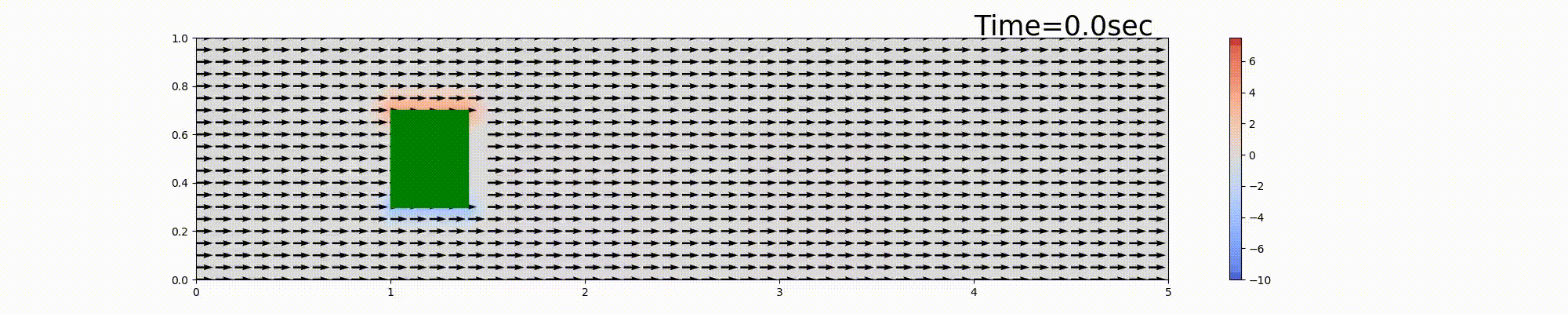
Figure 7.3 : Animation of calculation results (the flow velocity vector and the vorticity from the flow velocity)

7.6. About NaysMini

NaysMini is a solver that uses the Cartesian coordinate 2D model described in this chapter in conjunction with the iRIC GUI, and all of the source code is available. A NaysMini manual is also available. Please refer to it.