5. 1D unsteady flow with width variation

5.1. Basic equations

The previous chapter described a method for calculating 1D unsteady flow when the channel width is constant in the flow direction. This section describes the case where the channel width changes in the flow direction. When the channel width is constant, the unit width discharge \(q\) is used as the discharge, but here, we use the full flow discharge, \(Q\). The equation of motion and the equation of continuity for 1D unsteady flow in a channel with a general cross section are…

(5.1)\[{{\partial A}\over{\partial t}}+ {{\partial Q}\over{\partial x}}= 0\]

(5.2)\[{{1}\over{g A}}{{\partial Q}\over{\partial t}} +{{1}\over{g A}}{{\partial (A u^2)}\over{\partial x}} +{{\partial H}\over{\partial x}} + I_f =0\]

Where, \(t\) is the time, \(x\) is the distance in the flow direction, \(A\) is the cross-sectional area, \(Q\) is the discharge, \(g\) is the gravitational acceleration, \(u\) is the cross-sectional average velocity, \(H\) is the water level, and \(I_f\) is the energy gradient. Equation (5.1) is an equation of continuity for when the difference in discharge between the upstream end and the downstream end is equivalent to the temporal changes in the cross sectional area. Other terms than the first term, Equation (5.2) is the equation of continuity for steady flow. The first term expresses the temporal sequence of momentum.

The above equations are applicable to any cross sectional shape. Since the final goal is to apply the equations to 1D riverbed deformation, hereinafter the cross section is treated as rectangular. This means that the relationships of

(5.3)\[A=Bh, \ \ Q=Au=Bhu\]

are assumed to be satisfied, where, \(B\) is the channel width, \(h\) is the water depth, and \(H=h+z_b\), \(z_b\) is the riverbed elevation.

Taking into account of that \(h\) is a function of \(x\) and \(t\), and that \(B\) is exclusively a function of \(x\), (\(B\) does not change with time), then by using the relationship of Equation (5.3), we can transform Equation (5.1) and Equation (5.2) as follows.

(5.4)\[B{{\partial h}\over{\partial t}} + {{\partial (uBh)}\over{\partial x}} = 0\]

(5.5)\[{{\partial (uBh)}\over{\partial t}} + {{\partial (u^2 Bh)}\over{\partial x}}= -gBh{{\partial H}\over{\partial x}} -gBhI_f\]

The left side of Equation (5.5) is expressed in a form called “the conservation form”. This makes the equation applicable to a water surface with a discontinuous profile. When the water surface has a continuous profile, in other words when \(\displaystyle{{\partial h}\over{\partial x}}\) and \(\displaystyle{{\partial u}\over{\partial x}}\) are present, then the left side of Equation (5.5) is as follows.

(5.6)\[Bu{{\partial h}\over{\partial t}}+Bh{{\partial u}\over{\partial t}} + u{{\partial(Buh)}\over{\partial x}}+Buh{{\partial u}\over{\partial x}}\]

The equation can now be developed. Using the equation of continuity, (5.4), we transform Equation (5.5), as follows.

(5.7)\[{{\partial u}\over{\partial t}}+u{{\partial u}\over{\partial x}} = -g{{\partial H}\over{\partial x}} -gI_f\]

By applying the Manning formula to the energy gradient, \(I_f\), assuming a wide rectangular cross-section, and using the relationship of…

(5.8)\[u={1 \over n_m} h^{2/3} I_f^{1/2}\]

Equation (5.7) can be transformed as follows. Where, \(n_m\) is the Manning roughness coefficient.

(5.9)\[{{\partial u}\over{\partial t}}+u{{\partial u}\over{\partial x}} = -g{{\partial H}\over{\partial x}}-{{g n_m^2 u^2}\over{h^{4/3}}}\]

The following explanations use this non-conservation form of Equation (5.9) for the equation of motion. The non-conservation form of the equation of motion cannot usually address discontinuous flow. However, as was explained in the previous chapter, Equation (5.9) can be applied to discontinuous flows, to some extent.

5.2. Preparation for applying the CIP method (the split method)

Again, the basic formulas are…

(5.10)\[{{\partial h}\over{\partial t}}+ {1 \over B}{{\partial (uBh)}\over{\partial x}} = 0\]

(5.11)\[{{\partial u}\over{\partial t}} + u{{\partial u}\over{\partial x}} = -g{{\partial (h + z_b)}\over{\partial x}} -{{g n_m^2 u^2}\over{h^{4/3}}}\]

Calculate \(h\) with Equation (5.10), and \(u\) with Equation (5.11). Now, let us apply the split method to Equation (5.11). We split the equation as follows.

(5.12)\[{{\partial u}\over{\partial t}}= -g \displaystyle{\left( {{\partial h}\over{\partial x}} + {{\partial z_b}\over{\partial x}} \right) } -{{g n_m^2 u^2}\over{h^{4/3}}}\]

(5.13)\[{{\partial u}\over{\partial t}}+u{{\partial u}\over{\partial x}}=0\]

Note that the relationship of \(H=h+z_b\) is applied. In order to use Equation (5.11) to calculate \(u^n \rightarrow u^{n+1}\), we place \(\widetilde{u}\) in the middle, calculate \(u^n \rightarrow \widetilde{u}\) with Equation (5.12), and calculate \(\widetilde{u} \rightarrow u^{n+1}\) with Equation (5.13). Equation (5.12) includes \(h\). Therefore, when calculating Equation (5.12), Equation (5.10) must be satisfied at the same time. Let us express it \(h^n \rightarrow \widetilde{h}\). Equation (5.13) does not include \(h\). Therefore, it is impossible to relate it to Equation (5.10). For \(h^{n+1}\), \(\widetilde{h}\), the simultaneous solution to Equation (5.10) and Equation (5.12) is used as is, as follows.

(5.14)\[h^{n+1}=\widetilde{h}\]

The above is summarized in the table below.

Table 5.1 The split method for 1D unsteady flow

Phase name	Updating \(u\) and \(h\)	Equation used
[A] Non-advection Phase	\(u^n \rightarrow \widetilde{u}, h^n \rightarrow \widetilde{h}\)	Equations (5.12) and (5.10)
[B] Advection Phase	\(\widetilde{u} \rightarrow u^{n+1}, \widetilde{h} \rightarrow h^{n+1}\)	Equations (5.13) and (5.14)

5.3. The non-advection phase

First, we calculate \(u^n \rightarrow \widetilde{u}\) with Equation (5.12). At the same time, we perform \(h^n \rightarrow \widetilde{h}\). Then, Equation (5.12) is expressed as follows.

(5.15)\[{{\widetilde{u}-u^n}\over{\Delta t}}=-g \displaystyle{ \left( {{\partial \widetilde{h}}\over{\partial x}} + {{\partial z_b}\over{\partial x}} \right) } -{{g n_m^2 \widetilde{u}^2}\over{\widetilde{h}^{4/3}}}\]

Therefore, we obtain…

(5.16)\[\widetilde{u}= u^n - g \Delta t {{\partial \widetilde{h}}\over{\partial x}} - g \Delta t {{\partial z_b}\over{\partial x}} - g \Delta t {{n_m^2 \widetilde{u}^2}\over{\widetilde{h}^{4/3}}}\]

On the other hand, we calculate \(h^n \rightarrow \widetilde{h}\) with Equation (5.10). The following equation should be satisfied.

(5.17)\[{{\widetilde{h}-h^n}\over{\Delta t}} + {1 \over B} {{\partial}\over{\partial x}} (\widetilde{u} \widetilde{h} B ) =0\]

Therefore, simultaneous solutions to Equation (5.16) and Equation (5.17), i.e., \(\widetilde{h}\) and \(\widetilde{u}\), need to be obtained.

When the CIP method is applied to the calculation of a fluid, we use a “staggered grid”, in which the calculation points of \(u\) and \(h\) are alternatively arranged. Here, let us deploy the arrangement of calculation points shown in Figure 5.1.

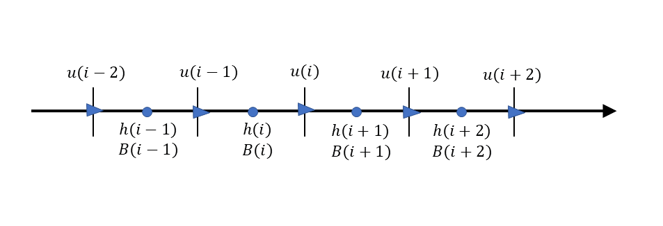
Figure 5.1 : Staggered grids

Taking into account the arrangement of calculation points in Figure 5.1, the difference expression of Equation (5.16) is as follows.

(5.18)\[\widetilde{u}(i) = u^n(i)-g\Delta t {{\widetilde{h}(i+1) - \widetilde{h}(i)}\over{\Delta x}} -g\Delta t {{z_b(i+1) - z_b(i)}\over{\Delta x}} - g \Delta t {{n_m^2 \widetilde{u}(i)^2}\over{\widetilde{h_p}^{4/3}}}\]

Where, \(\widetilde{h_p}=[\widetilde{h}(i)+\widetilde{h}(i+1)]/2\). To substitute this into the second term on the left side of Equation (5.16), we define discharge \(Q\) that satisfies…

(5.19)\[\widetilde{Q}=\widetilde{u} \widetilde{h} B\]

(the calculation points for \(Q\) are the same as those for \(u\).) Considering the arrangement of grid points, we have…

(5.20)\[\widetilde{Q}(i)= \widetilde{u}(i) {{\widetilde{h}(i+1)+\widetilde{h}(i)}\over{2}} B_u(i)\]

Where, \(B_u\) is the value of B at the calculation points of \(u\), and is expressed as…

(5.21)\[B(i)=\cfrac{B_u(i)+B_u(i-1)}{2}\]

The difference equation for Equation (5.17) that applies \(Q\) of Equation (5.20) is…

(5.22)\[\widetilde{h}(i) = h^n(i) + {1 \over B(i)} \left[ \widetilde{Q}(i)-\widetilde{Q}(i-1) \right] {{\Delta t}\over{\Delta x}}\]

We can obtain \(\widetilde{h}\) from this. However, because \(\widetilde{Q}\) on the right side of Equation \(bsa_7\) includes \(\widetilde{h}\) in negative form, repetitions of calculation are required. This procedure is shown in Figure 5.2.

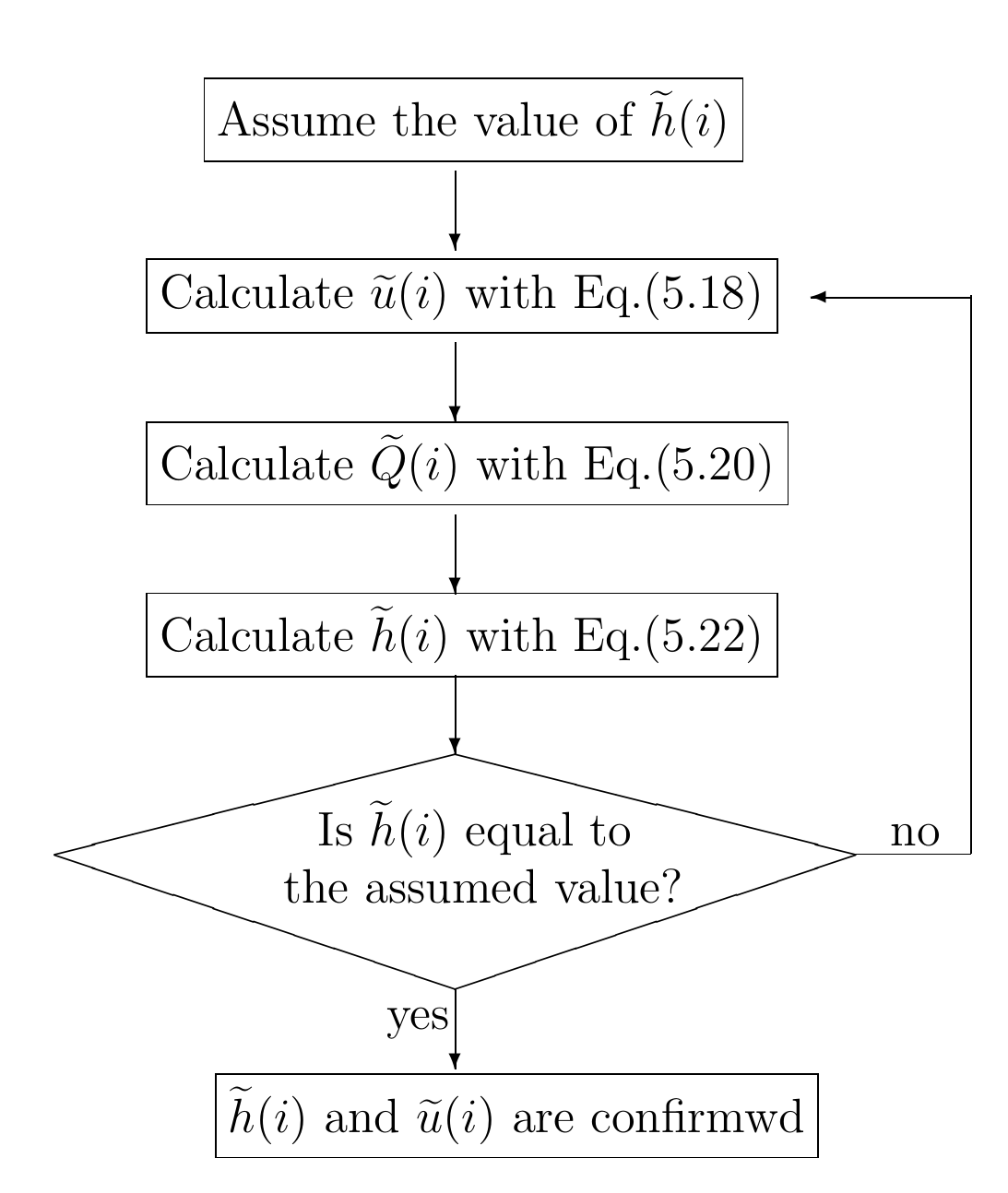
Figure 5.2 : The flow of the calculation procedure for, \(\widetilde{h}(i)\) and \(\widetilde{u}(i)\) in non-advection phase I

Once we obtain, \(\widetilde{u}(i)\) for non-advection phase, then we need to obtain \(\displaystyle{\widetilde{{\partial u}\over{\partial x}}}\) for non-advection phase. It can be obtained from the following equation, which is obtained by replacing \(f\) with \(u\) in Equation (3.38).

(5.23)\[\widetilde{{\partial u}\over{\partial x}}(i)= {{\partial u}\over{\partial x}}^n(i) +{{1}\over{2\Delta t}} \left[ \widetilde{u}(i+1)-u^n(i+1)-\widetilde{u}(i-1)+u^n(i-1) \right]\]

5.4. Advection phase

In the advection phase , the CIP method can be applied directly to Equation (5.13). Because this has been mentioned many times, here I give you only the results. They can be obtained by the following equation.

(5.24)\[{u(i)}^{n+1}=U(X)= \left[(aX+b)X+ \widetilde{{\partial u}\over{\partial x}}(i) \right] X +\widetilde{u}(i)\]

Where, \(\widetilde{u}(i)\) and \(\displaystyle{\widetilde{{\partial u}\over{\partial x}}(i)}\) are the spatial differentiation amounts of \(u\) and \(u\), respectively, in the non-advection phase. \(\displaystyle{\widetilde{{\partial u}\over{\partial x}}(i)}\) They are obtained from Equation (5.18) and Equation (5.22), respectively. \(U(X)\) is the spatial differentiation amount of \(u\) in the non-advection phase, given by the following equation.

(5.25)\[U(X)= \left[(aX+b)X+ \widetilde{{\partial u}\over{\partial x}}(i) \right] X +\widetilde{u}(i)\]

Therefore, using \(U(X)\), \(u\) in the advection phase, is given by…

(5.26)\[u(i)^{n+1}=U(X)\]

Similarly, the spatial differentiation amount of \(u\) in the advection phase is given by…

(5.27)\[\widehat{{\partial u}\over{\partial x}}(i) = 3aX^2 + 2bX + \widetilde{{\partial u}\over{\partial x}}(i)\]

and

(5.28)\[{{\partial u}\over{\partial x}}^{n+1}(i) = \widehat{{\partial u}\over{\partial x}}(i) -{{u(i+1)-u(i-1))}\over{2\Delta x}} \widehat{{\partial u}\over{\partial x}}(i) \Delta t\]

5.5. Summary

Flowchart Figure 5.3 summarizes the calculation of 1D free surface flow where the channel width varies in the downstream direction.

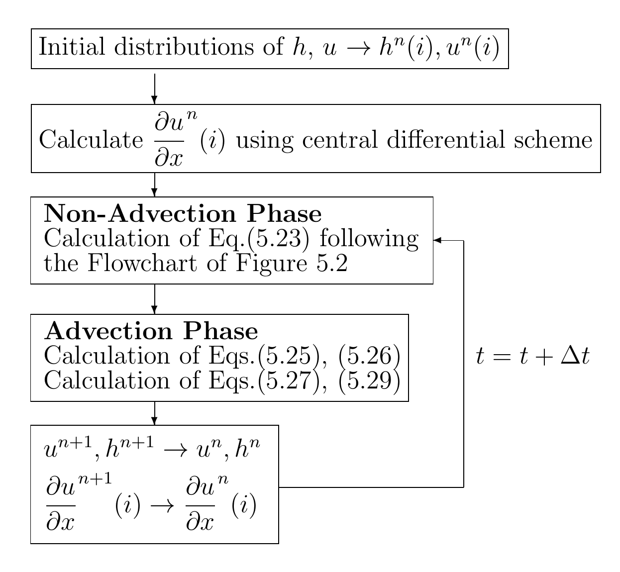
Figure 5.3 : The flow of calculation for flow with a 1D free surface

5.6. The Python code

An example of code for calculating the above 1D unsteady flow for a channel whose width varies in the longitudinal direction is below.

https://github.com/YasuShimizu/1D-Free-Water-Surface-with-Width-Variation

The files in this GitHub folder with the extension “py” are the calculation files. Of these, “main.py” files are those of the main body of the calculation code. Regarding the calculation conditions, [config.yml] is described below. Calculations can be carried out while changing the conditions by modifying the items in the comments as appropriate.

xl : 200 # channel length (m)
nx: 51  # number of grids in the x-direction
j_channel: 1 # condition of the channel (1 = constant gradient, 2 = gradient changes)
# when j_channel = 1
slope: 0.002 # entire gradient
# when j_channel = 2
x_slope : 100 # gradient changing point
slope1 : 0.001 # upstream gradient
slope2 : 0.01 # downstream gradient
xb1 : 90 # distance from the upstream end to the bump starting point (m)
xb2 : 100 # distance from the upstream end to the bump crest (m)
xb3 : 110 # distance from the upstream end to bump ending point (m)
dbed : 0. # bump height(m)
xw1 : 80 # location of channel width variation point 1 (m)
xw2 : 100 # location of channel width variation point 2 (m)
xw3 : 120 # location of channel width variation point 3 (m)
w0: 1 # channel width 1 (m) (upstream end)
w1: 1 # channel width 2 (m)
w2: 0.75 # channel width 3 (m)
w3: 1 # channel width 4 (m)
w4: 1 # channel width 5 (m) (downstream end)
qp : 1 # unit width discharge (m**2/2)
g : 9.8 # gravitational acceleration
snm : 0.025 # coefficient of roughness
alh : 0.6 # relaxation factor for water level calculation
lmax : 50 # max. replication number of water level calculation
errmax : 0.0001 # truncation error
hmin : 0.01 # min. water depth (m)
j_upstm : 2 # condition of upstream end (=wall, 2=free, 3=fixed value)
j_dwstm : 3 # condition of the downstream end
alpha_up: 1.0 # water depth at the upstream end (ratio over the neutral depth)
alpha_dw: 0.7 # water depth at the downstream end (ratio over the neutral depth)
etime : 400 # calculation end time (sec)
dt : 0.05 # calculation time step
tuk : 10 # output interval

The changes in channel width are assumed to be given by xw1, xw2, xw3, w0, w1, w2, w3, and w4. These parameters are explained in the figure below.

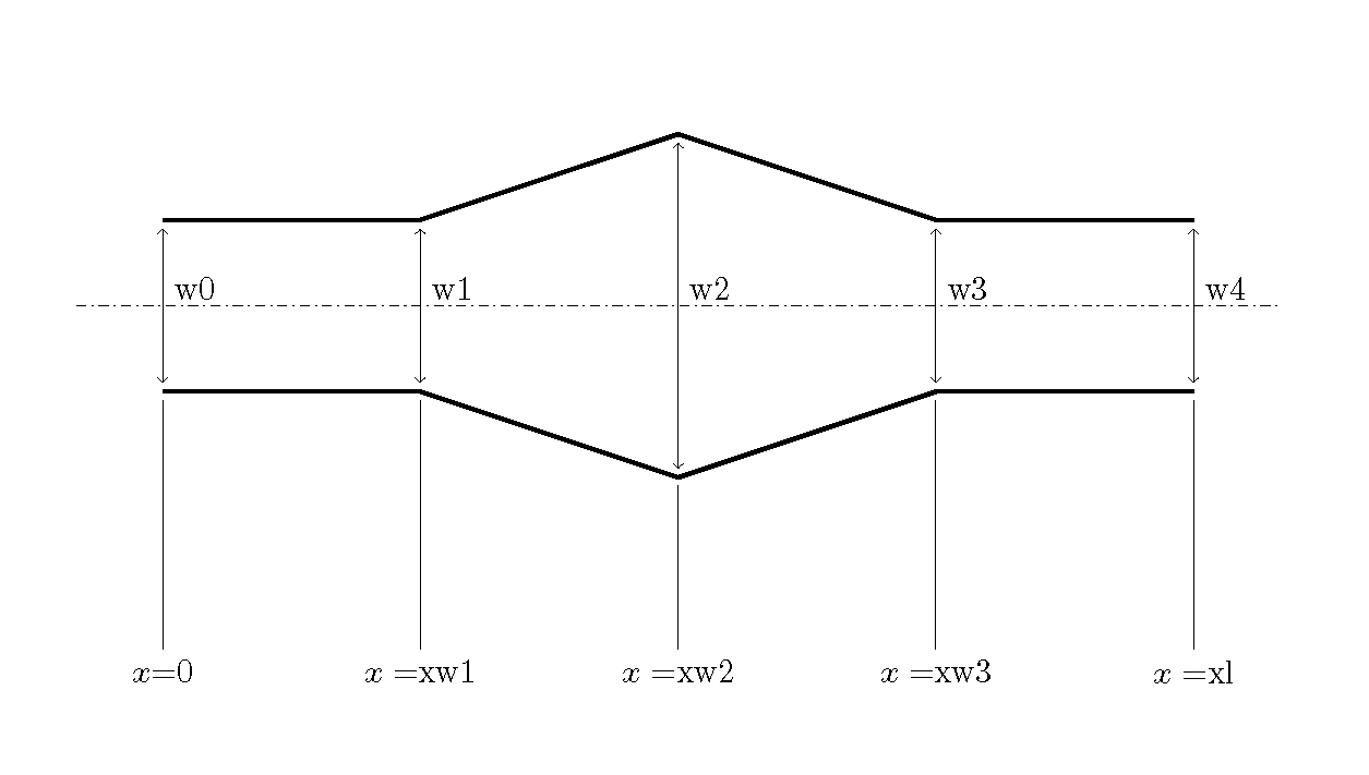
Figure 5.4 : Parameters for setting the channel width

5.7. A calculation example

5.7.1. Example of 1D flow calculation for a straight channel with a constriction

The figure below shows the calculation results for a channel whose width is 1m except for a constriction with a width of 0.75m at the longitudinal midpoint of the channel. In this example, a “drawdown” that is lower than the water depth of uniform flow is given to the downstream edge. The figure that shows the calculation results includes the uniform flow water level and the critical water level.

(5.29)\[h_0=\left(\cfrac{Q n}{B \sqrt{i}}\right)^{3/5}, \ \ h_c=\left(\cfrac{Q^2}{B^2 g}\right)^{1/3}\]

Figure 5.5 : A flow calculation example for drawdown in a channel with a narrow section at the longitudinal midpoint.