8. Basic knowledge on the alluvial river hydraulics
Note
In writing this section, Professor Yasuharu Watanabe of the Kitami Institute of Technology and Dr. Satomi (Yamaguchi) Kawamura, a Senior Researcher at the Civil Engineering Research Institute for Cold Region (CERI), provided images and video clips, as well as lots of advice. The following explanations owe greatly to their research achievements. I’d like to express my sincere appreciation to Professor Watanabe and Dr. Kawamura. Thank you very much!
Movable-bed rivers are those with sediment transport. Most rivers are movable-bed rivers. This section explains the minimum basic knowledge on the hydraulics of movable-bed rivers.
8.1. Riverbed and channel plane morphology
“Riverbed morphology” refers to the shape of the riverbed in a movable-bed river, while “channel morphology” refers to the geometric configuration. Riverbed morphology and channel morphology are topographies that form as a result of riverbed and riverbank evolution, such as from erosion and sedimentation at riverbeds and banks. The scale of these topographies are classified into small, medium, and large. The term “bed deformation” is sometimes used to refer to the combination of riverbed deformation and riverbank deformation.
“Small scale topography” is that on the scale of the grain diameter of bed materials. “Medium scale topography” is that on the scale of the water depth and river width. “Large scale topography” is that on the scale of the distance in the longitudinal direction of the river. For example, small-scale bed deformation means bed deformation at the particle-scale The riverbed morphology that emerges as a result of small-scale bed deformation is called “small-scale riverbed morphology”. It is also known simply as “bed waves”.
Bed deformation and channel/bed morphology are generally classified on the basis of scale, as follows.
The riverbed morphology has been classified by the Hydraulic Committee of the Japan Society of Civil Engineers (now the Committee on Hydroscience and Hydraulic Engineering) as follows [Ref:13].
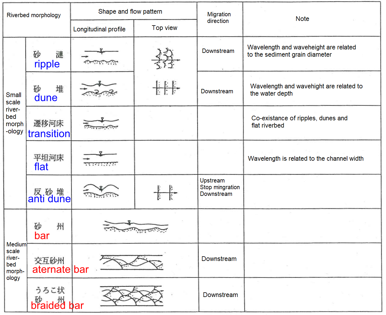
Figure 8.1 : Classification of riverbed morphology (Japan Society of Civil Engineers Engineers)
8.2. Basic features of small-scale bed morphology
Figure 8.2 represents the development of small-scale riverbed morphology proposed by Garcia [Ref:15]. According to this, we can see that the small-scale riverbed morphology changes (develops) with increase in the Froude number, \(F_r\). Note that flow with a low Froude number (approximately \(F_r < 0.8\)) is called the “lower regime”, and flow with a high Froude number (\(Fr>1.0\)) is called the “upper regime”.
The overall idea is that in a channel (river) that is initially flat with no sediment transport, the discharge gradually increases. Then, the process of changes in (the development of) the riverbed morphology is as follows. grain-scale ripples → mixed ripples and dunes → stable dunes → destabilized dunes → lost dunes and a flattened riverbed → flat-bed standing waves → anti-dunes A small-scale riverbed morphology is known to behave differently during development and during decay. This is called the “bivalence of resistance,” or the hysteresis phenomenon. The resistance (roughness) of a riverbed is highly dependent on the form of the small-scale riverbed morphology (bed waves). Therefore, it is extremely important to examine the small-scale riverbed morphology when calculating the coefficient of roughness for a river. For more information, refer to Kishi and Kuroki [Ref:32], or the like. This text briefly describes the roughness of flat riverbeds (when bed waves exert no influence) in Roughness of a flat riverbed.
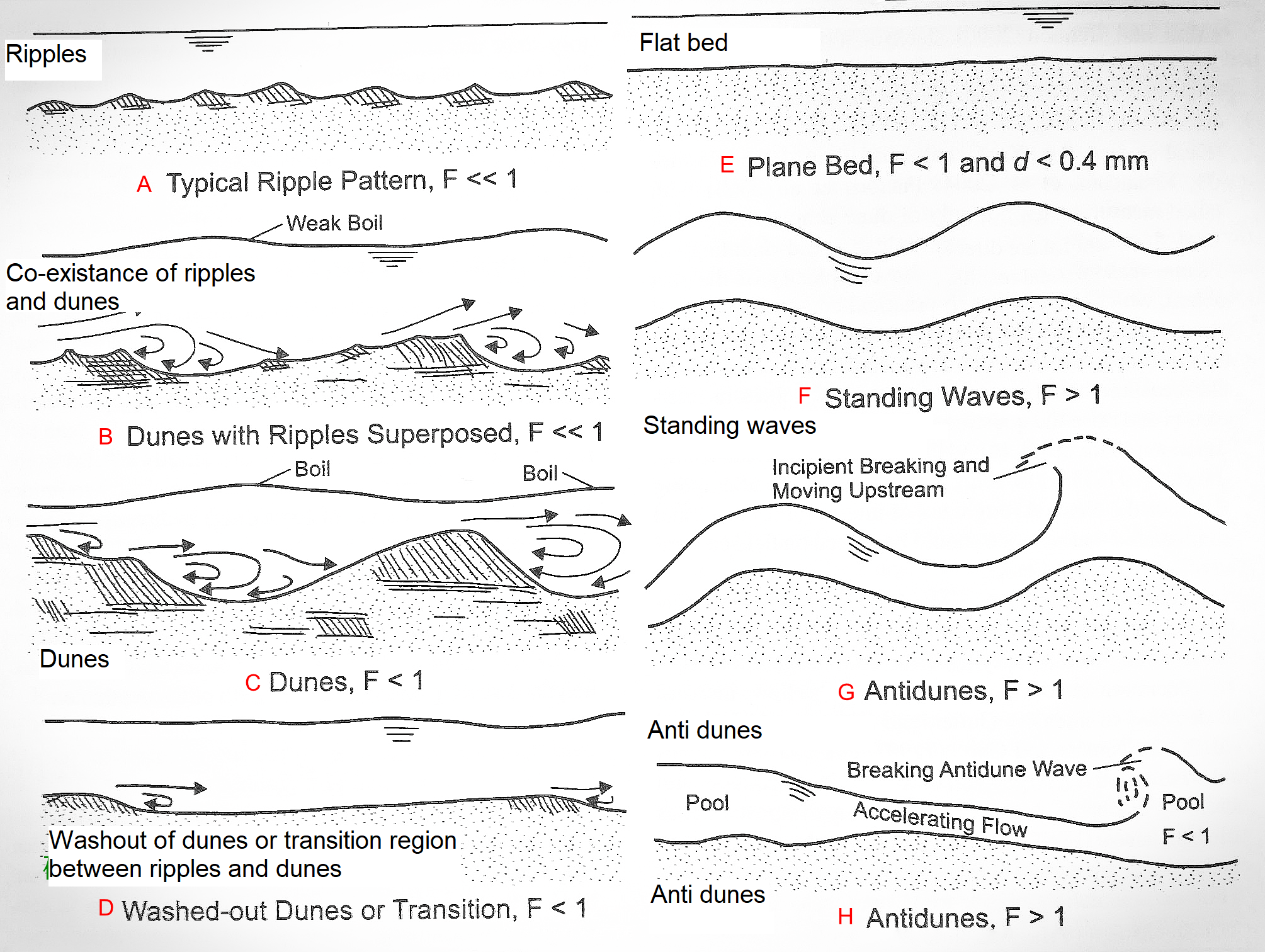
Figure 8.2 : Classification of small-scale riverbed morphology (Garcia [Ref:15])
According to [Ref:13], small-scale riverbed morphology (bed waves) is generally unstable, making it difficult to systematically sort out the characteristics of the wavelengths and wave heights. However, the following concepts are introduced.
8.2.1. The wavelength and wave height of the dune
According to the JSCE Hydraulic Committee [Ref:13], Figure 8.3 shows the relationship between the ratio of the mean water depth \(h\) to the wavelength of the ripples and dunes \(\lambda_s\) and the particle Reynolds number, \(u_\ast d_{50}/\nu\) for riverbed material when ripples and dunes are generated. Where, \(d_{50}\) is the 50% grain diameter, \(u_{\ast}\) is the shear velocity [refer to \(u_{\ast}\)], and \(\nu\) is the coefficient of kinematic viscosity of water. Consequently, the properties of \(h/\lambda_s\) change greatly at the boundary of \(u_\ast d_{50}/\nu \approx 20\). That is,
When \(u_\ast d_{50}/\nu > 20\), dunes are generated. \(h/\lambda_s\) is roughly constant and is \(\lambda_s \approx 5h\) on average.
When \(u_\ast d_{50}/\nu < 20\), ripples are generated, and \(h/\lambda_s\) changes greatly. There is no significant relationship between them.
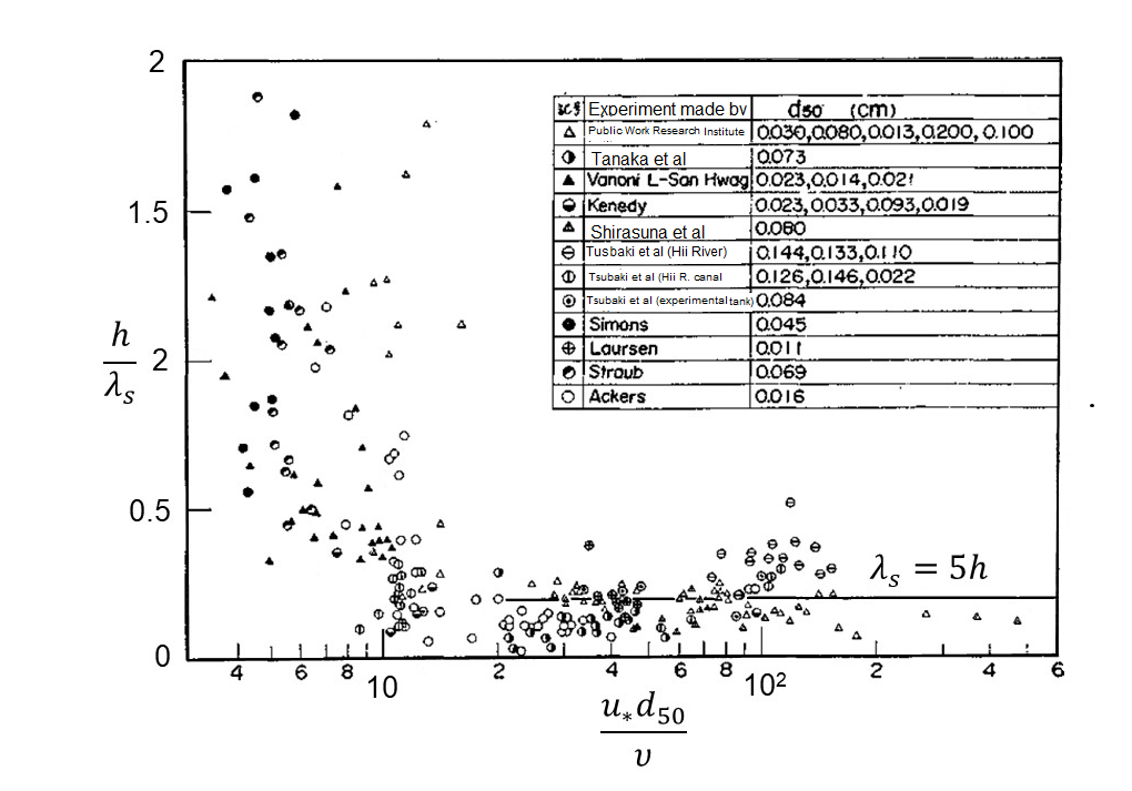
Figure 8.3 : Relationship between \(\cfrac{\Delta}{h}\) and \(\cfrac{u_\ast d_{50}}{\nu}\) regarding ripples and dunes (Hydraulic Committee of the Japan Society of Civil Engineers [Ref:13])
Regarding the wave length, \(\lambda_s\) and the wave height, \(\Delta_s\), Yalin [Ref:14] proposed the following equations.
Where, \(\tau_0\) and \(\tau_c\) are the shear stress and the critical shear stress, respectively. They will be explained in the next section. From Figure 8.3, we can assume that Equation (8.1) is satisfied. The relationship between \(\Delta_s/h\) and \(\tau_c/\tau_0\) is as shown in Figure 8.4. The range of the parameter of Equation (8.2) is \(1/6 \sim 1/2\).
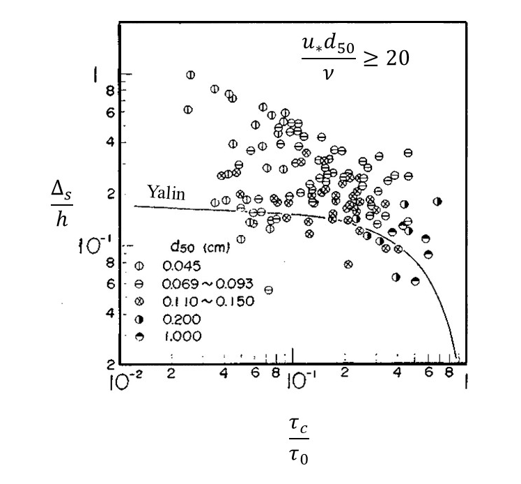
Figure 8.4 : Relationship between \(\cfrac{\Delta_s}{h}\) and \(\cfrac{\tau_c}{\tau_0}\) of ripples
In (8.2), when \(\tau_0\) is significantly larger than \(\tau_c\), then we have…
When sediment transport is great, the wave height of the dune reaches about 20% of the water depth. In this condition, the dune migrates at a constant velocity.

Figure 8.5 : Video clip of dune migration in an experimental channel [Ref:17]
Figure 8.5 is a video clip of a dune migration experiment conducted by Inami et al. of CERI ([Ref:17]). The experiment was made using a tank with a channel width of 0.5 m, a gradient of 1/500, and sand with a uniform grain diameter of d \(_m\) = 0.515 mm. The discharge was 30 \(\ell/s\). This video shows a longitudinal visual field of approximately 5.5 m. The water depth read from the video is about 20 cm, the wavelength of the dunes is about 1 m, and the wave height of dunes is about 4 cm. As you can see, the experimental result matches Equation (8.1) and Equation (8.3).
8.2.2. Wavelength and wave height of ripples
The wavelength and wave height of ripples are related to the grain diameter rather than to the water depth. In general, their relationship is as follows [Ref:13].
8.3. Basic features of mesoscale bed morphology
According to Watanabe [Ref:18], the mesoscale riverbed morphology refers to landforms on the scale of the river width that formed on the riverbed (the “raiagaku” pattern). Based on their shape, the landforms are classified as (a) alternate bars (single-row bars), (b) double-row bars, or (c) multi-row bars (braided bars). Areas of scouring and accretion appear, triggering meandering flow, which in turn leads to local scouring and riverbank erosion. Therefore, these are important phenomena for flood control in terms of maintaining the river channel, and they are important phenomenon for the river environment because of their relation to riffles and pools, which are important environmental elements of rivers. They have attracted the attention of river engineers from the olden days.
8.3.1. Alternate (single-row) bars
When alternate bars (single bars) are generated, the flow meanders, scouring and deposition occur on the left and the right banks alternately, a clear front edge of bar arises that shows the shape of the bar, and the bar begins to progress downstream with time (Figure 8.6).
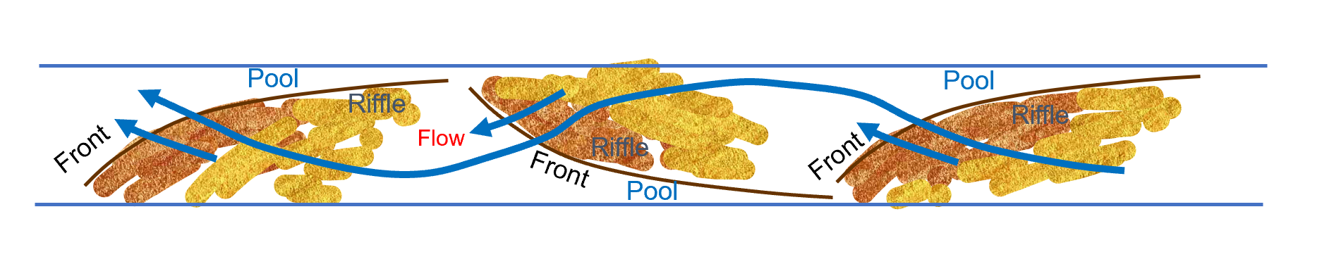
Figure 8.6 : Schematic of single-row bars
Professor Watanabe of the Kitami Institute of Technology has given the following explanation of the front edge of bar. [Ref:19]
Note
On a riverbed where bars have formed, the sediment transport stops at certain points and causes shoulders to form on the mound. These shoulders are present in the form of an arc in the plane of the riverbed, as seen in the figure below (Figure 8.7). They advance downstream with increasing height and develop to a certain height. After this development, the arc-shaped shoulder of the mound continues to advance downstream. This arc-shaped sedimentary shoulder is called the front edge of bar.
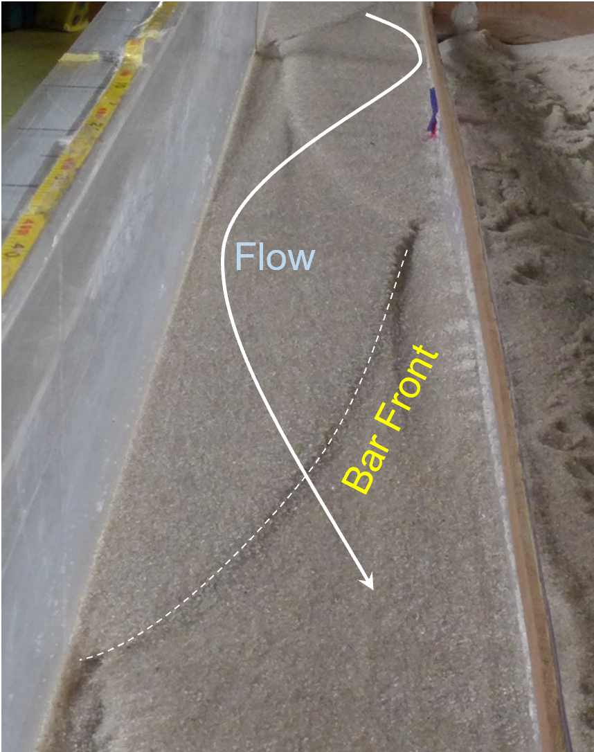
Figure 8.7 : Diagram defining the front edge of bar [Ref:19]
Figure 8.8 is a video of the top view of an experiment conducted at CERI on the movement of alternate bars in a straight channel [Ref:20], where, the channel width \(B=\) is 0.9 m, the bed gradient \(i=\) is 1/200, the mean grain diameter of bed material \(d_{50}=\) is 0.77 mm, and the discharge is \(Q=8 \ell\) /s.
Figure 8.8 : Video clip of the migration of alternate bars in a straight channel [Ref:20]
Figure 8.9 Is calculated under the same experimental conditions as Figure 8.8, and was calculated with Nays2dH of iRIC. The calculation results also show that the alternate bars that were generated migrate in the same way as those of the experimental results.
Figure 8.9 : Calculation results for the migration of alternate bars in a straight channel.
8.3.1.1. Naka River
The alternate bars in the Naka River (Figure 8.10) are well-known as alternate bars in an actual river.
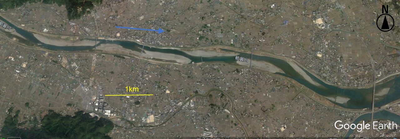
Figure 8.10 : An example of alternate bars (Naka River), Source from Google Earth
8.3.1.2. Tokachi River
The new straight channel section of the Tokachi River has clear alternating bars, as shown in Figure 8.11.
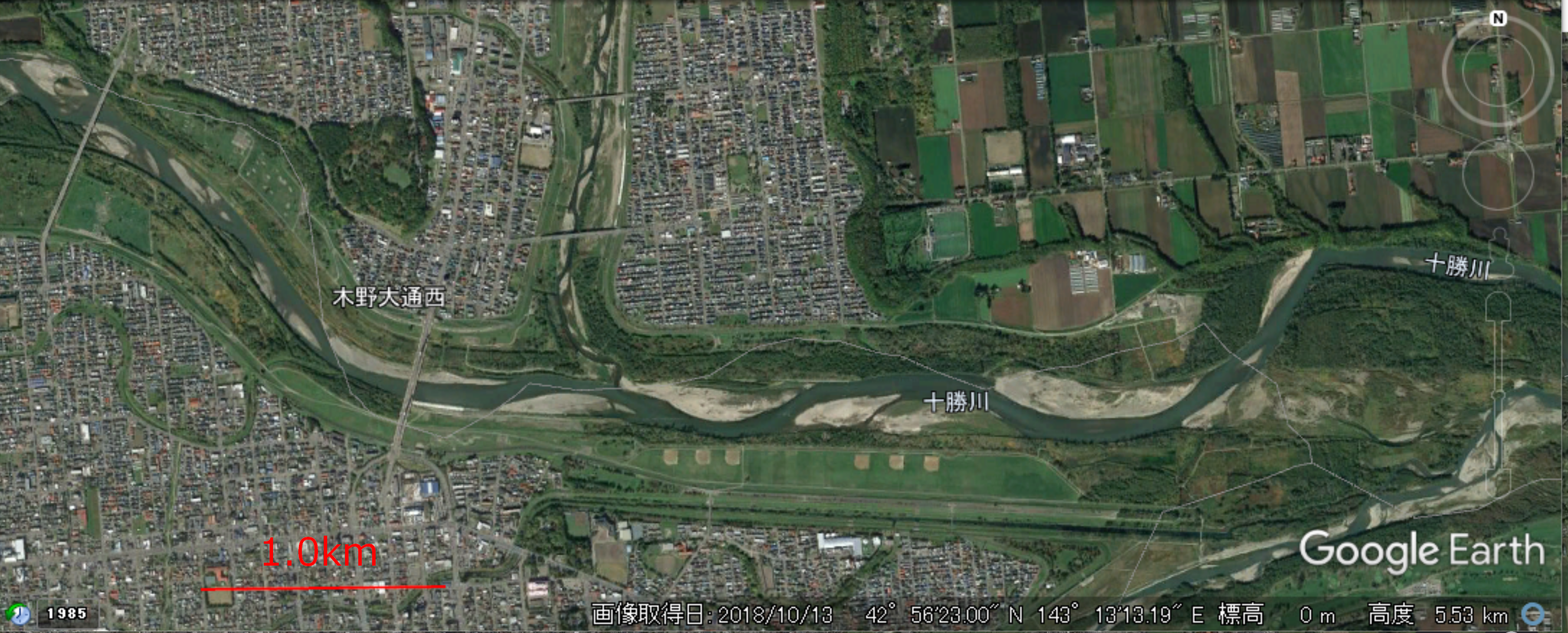
Figure 8.11 : An example of alternate bars (Tokachi River)
Aerial video clip of single-row bars in the Tokachi River (shot by drone on Nov. 9, 2021)
8.3.2. Double-row bars
The river morphology is described as “double-row bars” when all of the following are met: 1) two rows of single-row bars are generated in the cross-sectional direction, 2) bed scouring and accretion occur alternatively along both banks and along the center of the channel in the longitudinal direction, and 3) the flow forms a figure eight. Although double-row bars also progress downstreamward, they migrate at velocities lower than those of single-row bars (Figure 8.12).
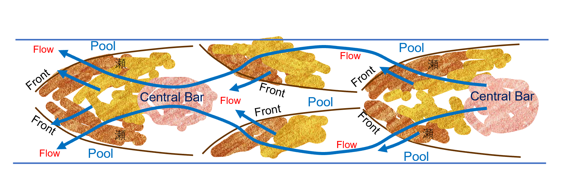
Figure 8.12 : Schematic of double-row bars
8.3.2.1. Sho River
Figure 8.13 is an example of double-row bars that developed in the Sho River in Toyama Prefecture, Japan.
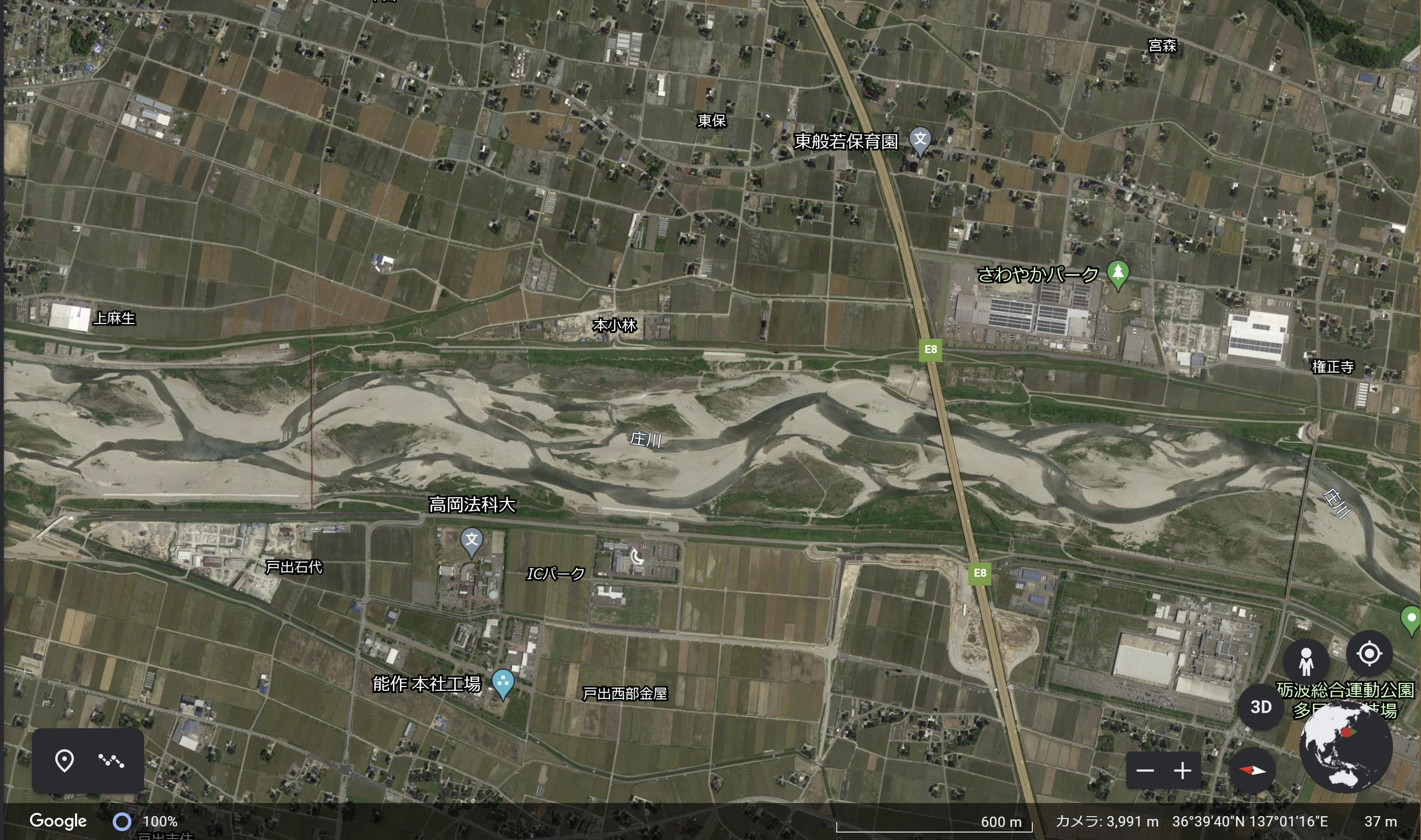
Figure 8.13 : An example of double-row bars (Sho River) from GoogleEarth
Aerial video clip of double-row bars in the Sho River (shot by drone on Oct. 28, 2021)
8.3.2.2. Satsunai River
These are double-row bars in the Satsunai River. (Figure 8.14)
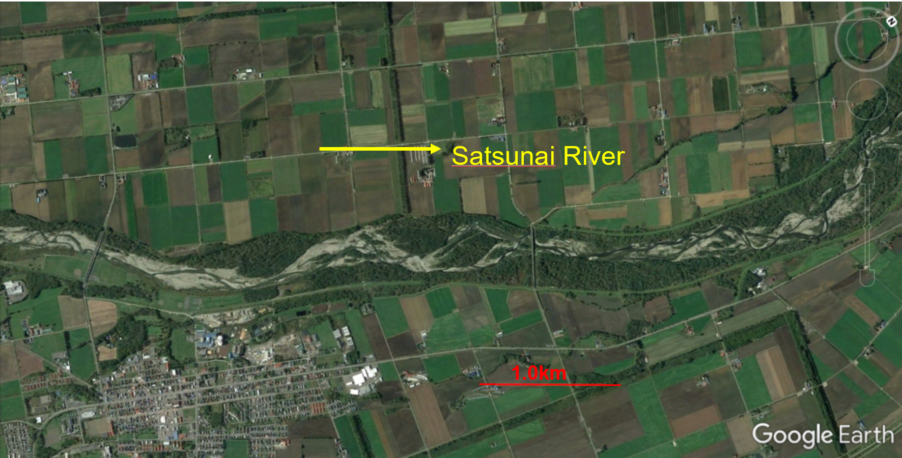
Figure 8.14 : Section of the Satsunai River with double-row bars
Aerial video clip of double-row bars in the Satsunai River (shot by drone in June 2019). Video courtesy of the Obihiro Development Construction Dept. of the Hokkaido Regional Development Bureau.
Aerial video clip of double-row bars in the Satsunai River (shot by drone in Nov., 2021). Video courtesy of Hokkaisuiko Consultant Corp.
8.3.3. Multi-row bars (braided bars, scaly bars)
The number of rows of bars in the cross-sectional direction of a channel is called the mode number. bars with a mode number of three or more are called multi-row bars, braided bars or scaly bars.
8.3.3.1. Oi River
Figure 8.15 is an example of braided bars in the Oi River in Shizuoka Prefecture, Japan.
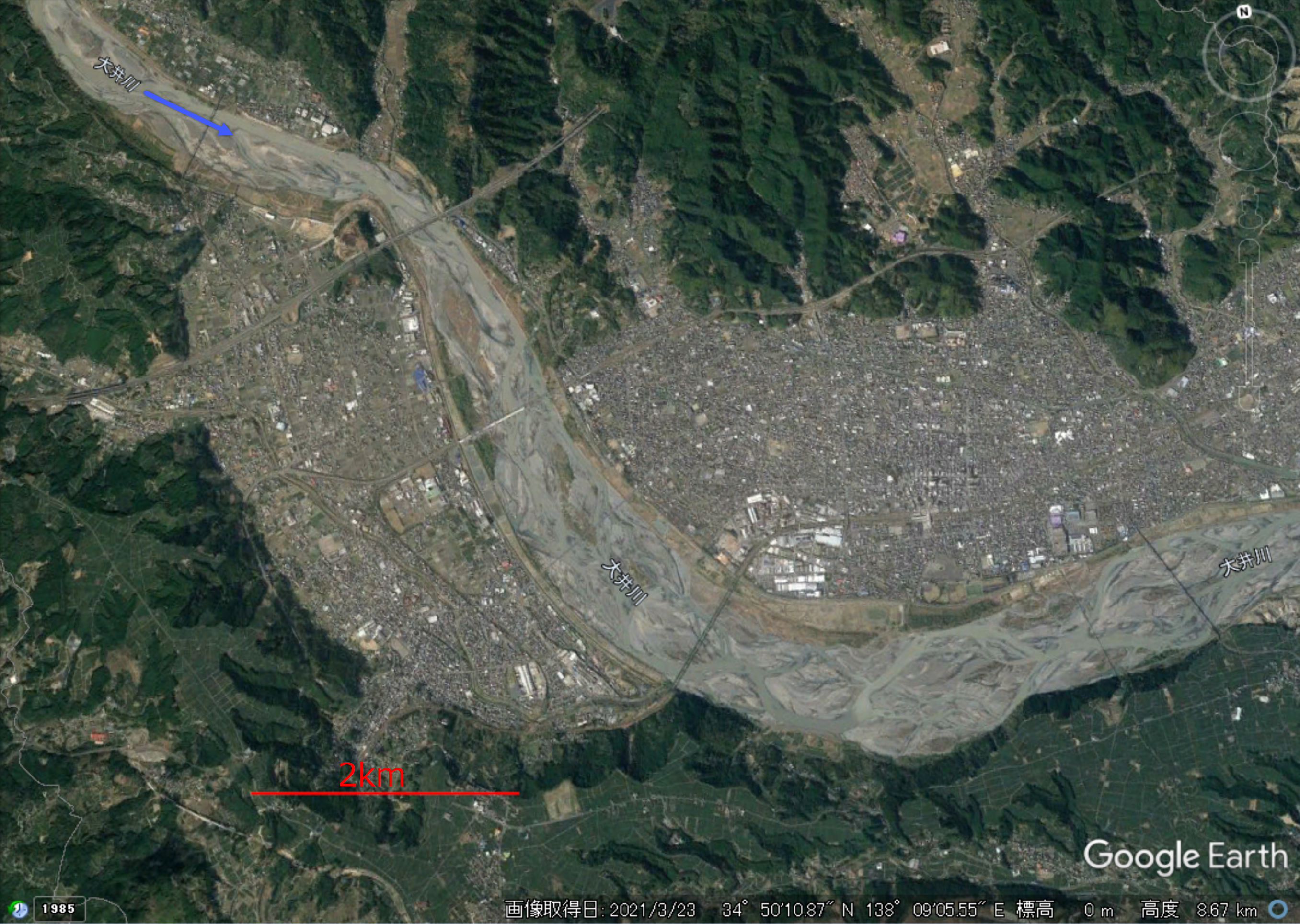
Figure 8.15 :An example of braided bars in the Oi River from Google Earth
Aerial video clip of double-row bars in the Oi River (shot by drone in Sept. 2022); Video courtesy of Kazutake ASAHI (RiverLink Co., Ltd.)
8.3.3.2. Hii River
Figure 8.16 is an example of braided bars in the Hii River in Shimane Prefecture, Japan.
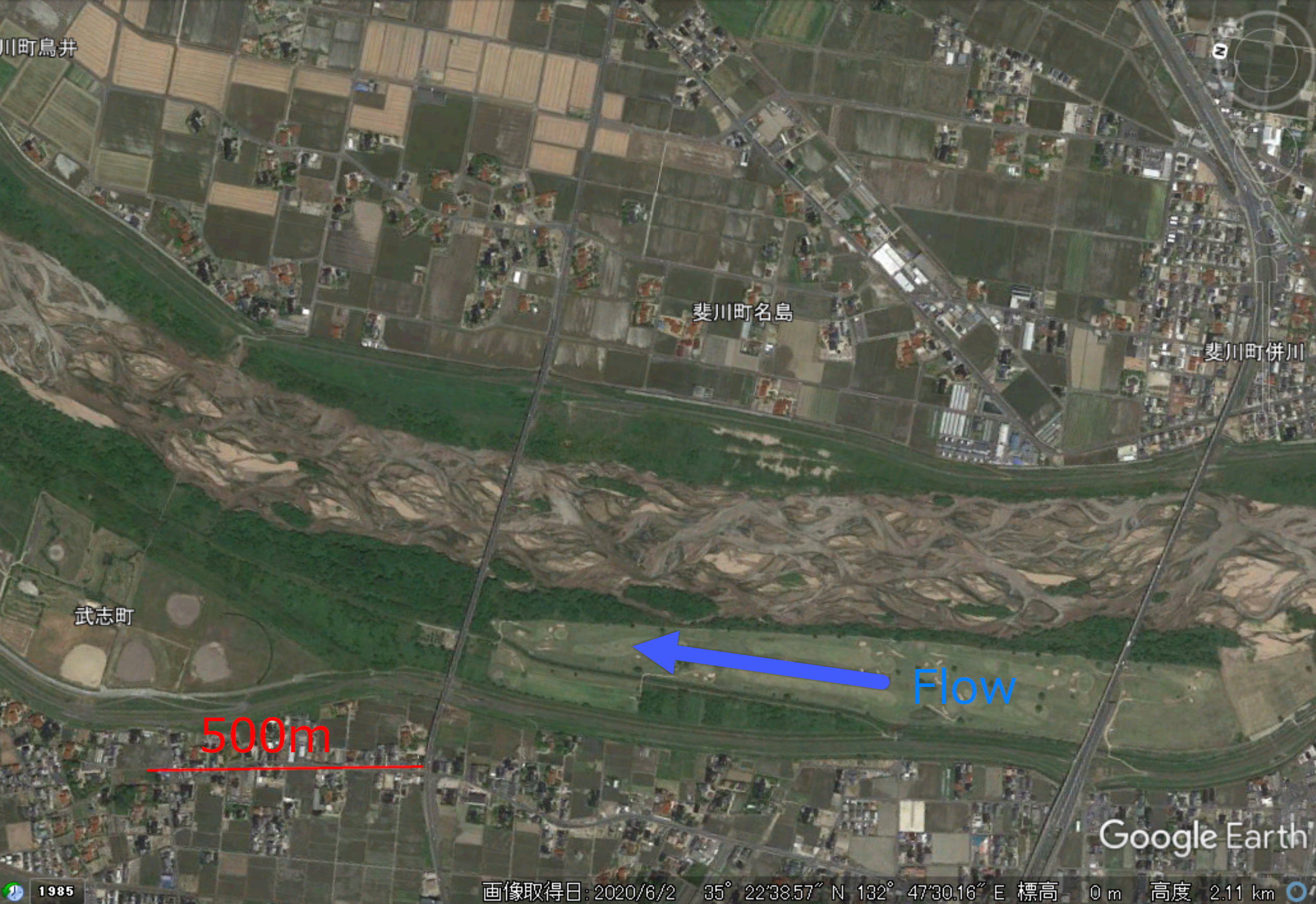
Figure 8.16 :An example of braided bars in the Hii River from Google Earth
Aerial video clip of double-row bars in the Hii River (shot by drone on Dec. 3, 2021) [Ref:36]
8.3.3.3. Braided rivers around the world
8.3.4. Regime criteria of the mesoscale bed morphology
Researchers have spent many years how to classify the region of bar emergence, i.e., the geometric and hydraulic conditions of a channel that generate certain type of bars. The region is known to depend on the ratio of the channel width to the channel depth (\(B/h\)). One method of theoretical analysis is called linear stability analysis. A drawing developed by Kuroki and Kishi [Ref:21] for practically classifying which regions cause bars of which type to develop is often used in Japan. Figure 8.17 is made by plotting data from an experimental channel on a drawing for classifying a region. Here, the parameter on the horizontal axis, \(\cfrac{BI^{0.2}}{h}\), allows us to include the effects of gradients, to a small extent, how gradients affect the ordinary channel width and water depth data. This enables us to classify rivers with a wide range of gradients by using a single drawing for classifying a region. The river width and water depth of this parameter are the channel width and mean water depth for an experimental channel, respectively. For an actual river, it is recommended to use the bankfull discharge in the low-water channel or the water depth and the water surface width at the time of the mean annual maximum discharge.
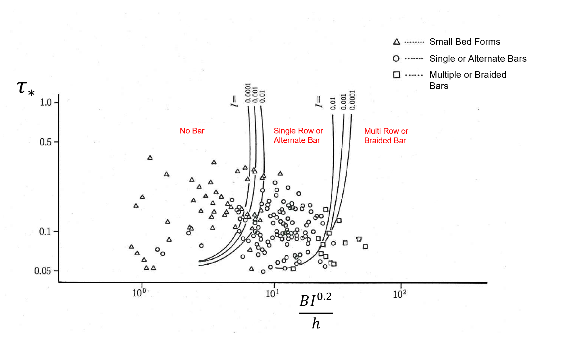
Figure 8.17 : Classification of the regions of mesoscale riverbed morphology by Kuroki and Kishi (comparison with experimental channel data) [Ref:21]
Figure 8.18 was made by plotting data from actual rivers recorded by Yamaguchi and Kuroki [Ref:22].
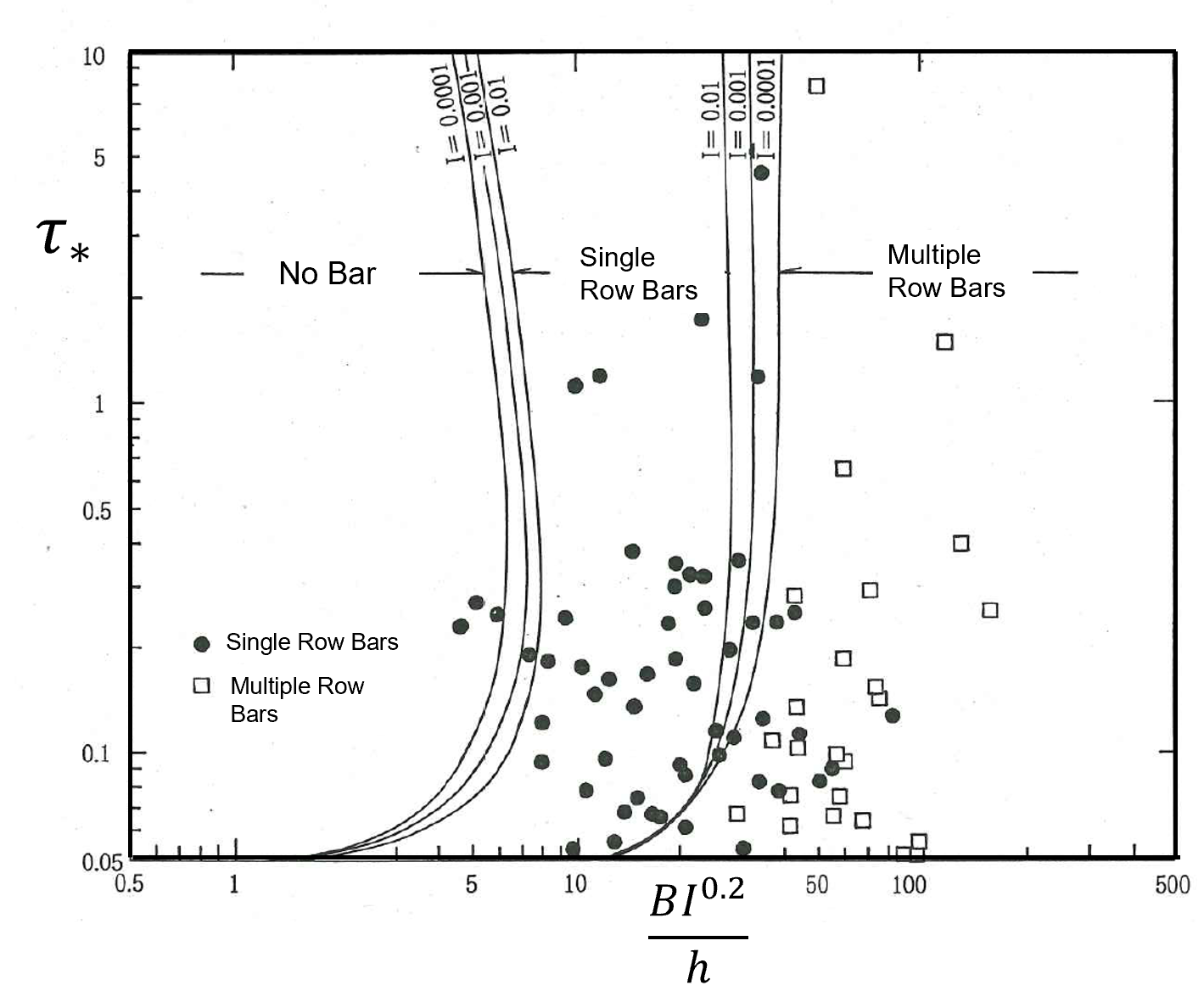
Figure 8.18 : Classification of regions of mesoscale riverbed morphology by Kuroki and Kishi (comparison with actual river data) [Ref:22]
8.3.5. Basic features of mesoscale bed morphology
The bar wavelength for a riverbed with a mesoscale morphology has a high correlation with the river width (channel width). According to Figure 8.19 in [Ref:13], they are distributed in the range shown in…
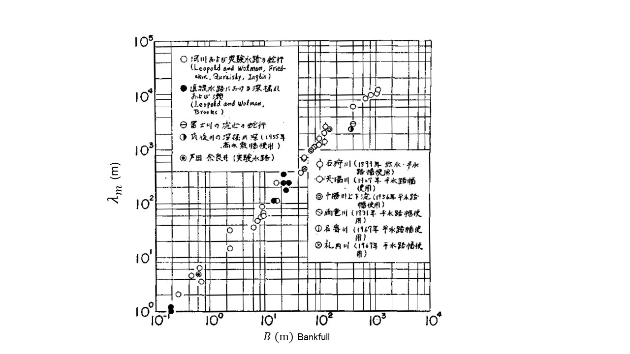
Figure 8.19 : Relationship between bar wavelength and river width
Where, \(\lambda_b\) is the wavelength and \(B\) is the river width. For an actual river, \(B\) is the surface water width of the low-water channel at the time of bankfull discharge in the low-water channel. For an artificial watercourse, it is the channel width. Note that the bar wavelength here differs from the meander wavelength described later.
bar wave heights also have high correlations with \(B/h\). Here, we introduce the bar wave height of the single-bar equation, Equation (8.7), developed by Ikeda [Ref:23].
Where, \(Z_B\) is the bar wave height, and \(d\) is the grain diameter of the bed material.
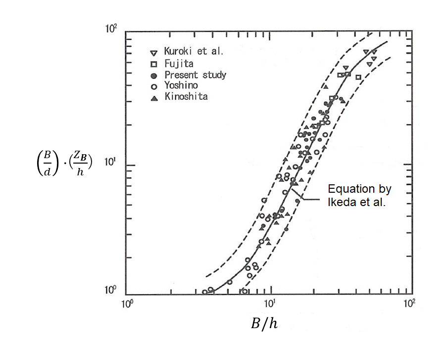
Figure 8.20 : bar wave height data and the equation developed by Ikeda [Ref:23]
8.4. Plane morphology of the meandering rivers
For natural rivers on alluvial land, the riverbanks are subject to be eroded by the river flow, which also changes the plane shape of the river. A typical river plane shape is a meander, where the flow channel swings from side to side. The causes of meandering are explained by two hypotheses. (1) The plane shape instability hypothesis: The instability of river plane shape itself causes the river to meander. (2) The bar-induction hypothesis: The generation of alternate bars initiates river meandering.
8.4.1. Meandering caused by bars
When alternate bars occur in a river, the flow is deflected leftward or rightward, and erosion occurs alternately on the left and right banks. This causes the stream channel itself to begin to meander. Figure 8.21 is a schematic diagram produced by Kinoshita [Ref:24] showing how the development of a bar leads to the meandering of the river channel, and then to a plane shape with a higher degree of meandering, also called “great meander” or a “tortuous meander”.
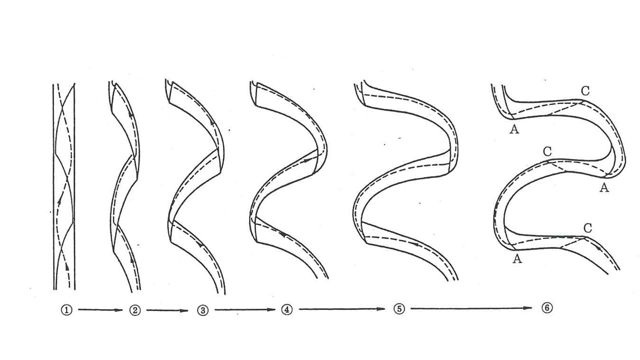
Figure 8.21 : Schematic by Kinoshita [Ref:24]: explanation of how bars develop into meanders
The following is an explanation by Kinoshita [Ref:24] on the process of meander development
Alternate bars form in the straight river channel, and the flow meanders. (There are single-row bars and double-row bars.)
In the early stages of meandering, the meander consists of two bars, the centroid moves downstream of the concave bank side, and the meander of the channel progress downstreamward (a meandering river channel).
As the meandering progresses, the number of bars in each meander increases from two to three, and the centroid can be located not only downstream of the concave bank, but also laterally and upstream of the concave bank. This allows a meandering shape to develop in the lateral and upstream directions. This leads to the formation of a spur, such as at point A in ⓺ (a “great meander”, or a “tortuous meander”).
As the meandering progresses, the area near point A eventually becomes an immovable point. It is overtaken by the advancing meandering channel, finally leading to a natural short-circuit.
Meandering that becomes so severe that more than one pair of bars form within one wavelength of meandering is called a “grate” (or “tortuous”) meander. When bars cause the turning point of the curvature of a meandering streamline to be located at the outer bank of a river bend of the channel plane shape, that turning point is called a B-type connection, whereas when bars cause such a turning point to be at the inner bank of a bend, the connection is called a C-type connection. Menders develop when there are B-type connections, and stop developing when there are C-type connections (Figure 8.22).

Figure 8.22 : Connection of bars in a tortuous meander (Figure transcribed from [Ref:18] by Watanabe).
8.4.2. Menders caused by plane shape instability
Ikeda et al [Ref:25] regarded that the mender induced deviation velocity provides the driving force of bed variations, and used Engelund’s theoretical solutions for meander flow to derive the conditions under which the plane shape becomes unstable, and to obtain the dominant wavelength. This was the first study on the plane shape instability hypothesis of meanders. Since then, similar studies on meanders that develop from plane shape instability have been carried out by different researchers. However, the above-mentioned influence of bars has not been included, and subsequent studies have reported that meanders can develop even without the influence of bars ([Ref:26]).
8.5. Free bars and point bars
Up to this point, bars have been classified as single-row or double-row bars. There is another method of classification. It uses the classification of “free bar” and “point bar”. Free bars occur in straight or nearly straight rivers and progress freely downstreamward, whereas fixed bars are defined by the channel plane shape(meander shape) and emerge on the inner bank of a bend at fixed locations.
As you can see, the bars that were generated in the aforementioned experiment by CERI (Figure 8.8) and those that were reproduced by the verification calculation of the experiment (Figure 8.9) are migrating bars. Therefore, they are free bars. The alternating bars of the Nagawa River (Figure 8.10) and the double-row bars of the Shogawa River (Figure 8.13) and Hiigawa River (Figure 8.16) are also considered to be free bars.
8.5.1. Critical meander angle for bar progress
According to Kinoshita [[Ref:24], as shown in Figure 8.23, when \(\theta\) (the meander angle) shown in the figure exceeds a critical angle, the bar stops migrating forward and becomes a bar whose shape is a combination of an alternating bar and a fixed bar.
Figure 8.23 : Critical angle at which a bar stops migrating (Kinoshita [Ref:24])
The definition of meander angle in Figure 8.23 is that for a zigzag channel. For ordinary rivers, the meander angle is defined as the angle at the point where the angle between the valley axis and the channel centerline is the maximum, as shown in Figure 8.24, and it is called the meander angle or the maximum meander angle.
Figure 8.24 : Definition of meander angle
In the following Figure 8.25 \(\sim\) Figure 8.28 are the bed deformation simulation results when the hydraulic conditions other than the meander angle are kept the same and the meander angle is varied in the range of \(0^{\circ} \sim 30^{\circ}\). Bars that move freely downstream in a straight channel slow down with each increase in meander angle, as if constrained by the topography. You can see that the bars completely stop at \(30^{\circ}\) in Figure 8.28. This is consistent with the point made by Kinoshita [Ref:24]. The calculation model used here is Nays2dH of iRIC and it is the same model as Hasegawa [Ref:27] used for experiments on a straight channel and on alternating bars.
Figure 8.25 : Simulation of bar migration in a straight channel
Figure 8.26 : Simulation of bar migration when the mender angle is \(\theta=10^{\circ}\)
Figure 8.27 : Simulation of bar migration when the mender angle is \(\theta=20^{\circ}\)
Figure 8.28 : Simulation of bar migration when the mender angle is \(\theta=30^{\circ}\)
8.5.2. Gourd-shaped river channel (a river characterized by narrow and wide sections repeating periodically)
It would be interesting to know whether six different mesoscale riverbed configurations exist. They would be the combinations of any of the following three items (A) no bars, B) single-row bars or C) double-row bar) with either 1) free bars or 2) fixed bars, i.e., 3×2 combinations. This is still an open area.
First, it is easy to imagine that (B-1) and (C-1) can occur when the channel is nearly straight and the hydraulic conditions are within the region of bar generation. (However, it is debatable, especially in the case of a double-row free bar, whether the conditions continue until the state of dynamic steady state.) Next, (B-2) is an example of alternate bars that have been trapped in a channel plane shape. Such bars occur when the meander angle of the alternating bar exceeds the critical angle. In this case, free bars and fixed bars are considered to coexist. The question is whether (C-2) exists. This is equivalent to the rivers characterized by narrow and wide sections existinging periodically reported by Watanabe et al. [Ref:28] and Yamaguchi and Watanabe [Ref:29]. Such channel forms are found in natural rivers such as the Hii River and the Satsunai River.
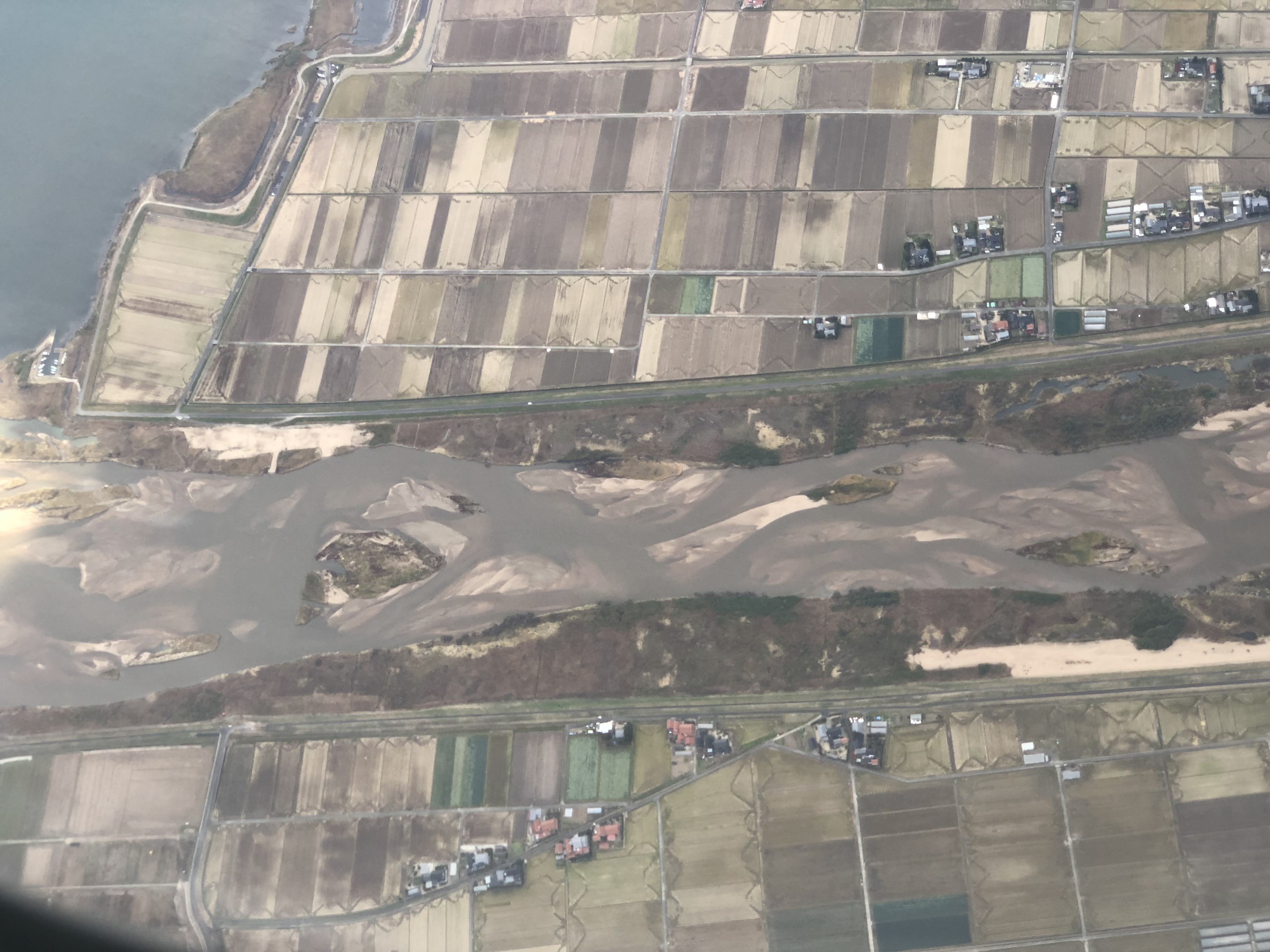
Figure 8.29 : Hii River estuary, with a channel with repetitions of narrow parts (nodes) and wide parts (anti-nodes) (December 4, 2021, taken from a JAL aircraft just after takeoff from Izumo Airport).
8.6. Examples of meandering rivers
Almost all natural rivers meander, so it is extremely easy to find meandering rivers on Google Earth or other tools. For example…
8.6.1. Shimanto River
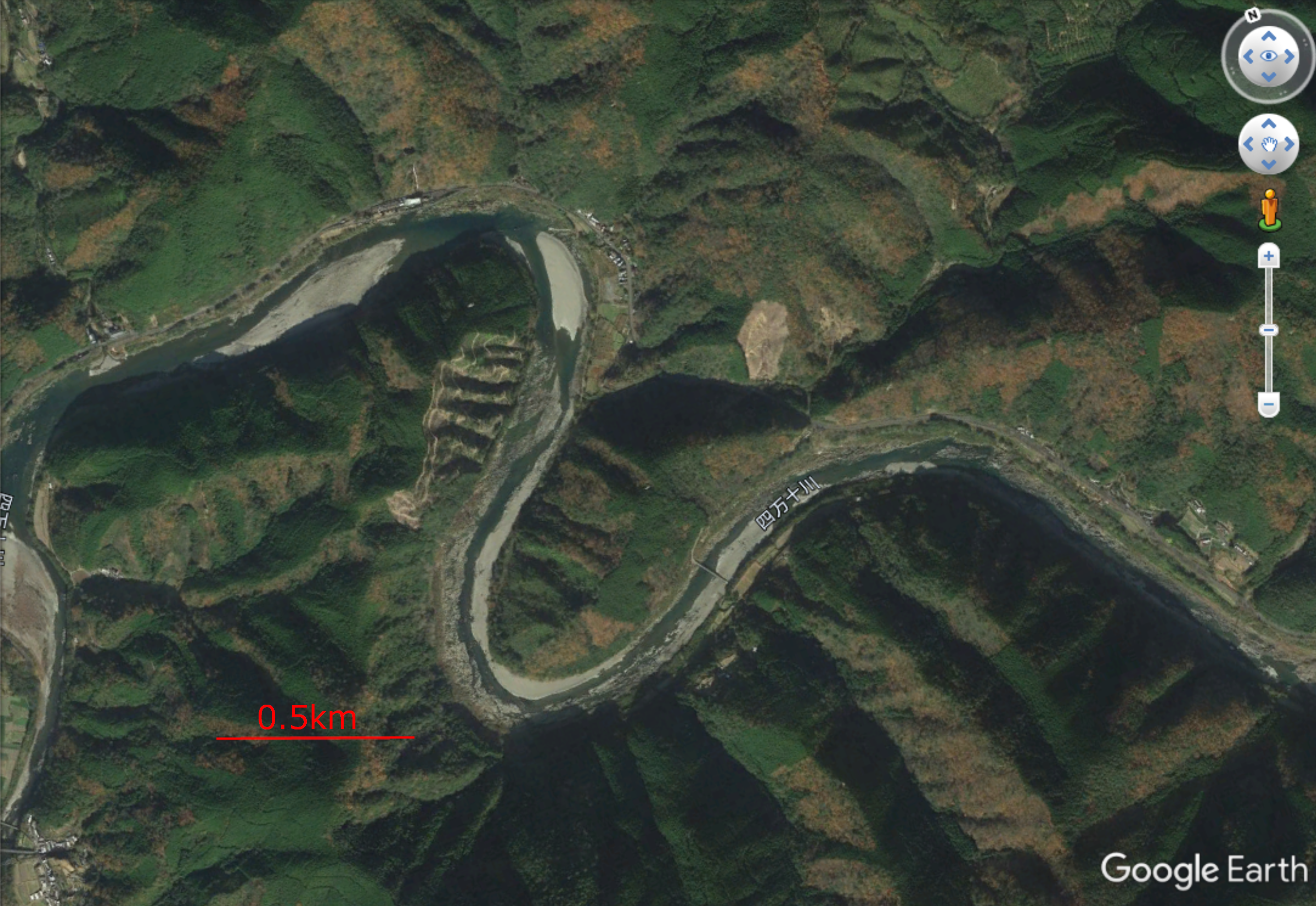
Figure 8.30 : Meanders and fixed bars in the Shimanto River, Kochi Prefecture
8.6.2. Sorachi River
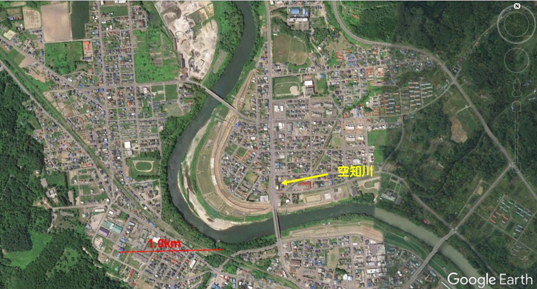
Figure 8.31 : Fixed bars at the bend of the Sorachi River, Hokkaido Prefecture
Google Earth Engine now allows anyone to study the evolution of channel plane profiles on meandering rivers over the past several decades.
8.6.3. Ukayari River
Figure 8.32 : Free meandering of the Ukayari River in the upper Amazon basin (Peru)
8.6.4. Ichilo River
Meandering of Bolivian rivers in the upper Amazon basin over a period of 30 years (created by Google Earth Engine) [Ref:16]
It is now possible to simulate the long-term temporal variation of free meandering. Following Figure 8.33 is the result of numerical simulation of free meandering by Asahi et al [Ref:30].
Figure 8.33 : Simulation of free meandering by Asahi et al [Ref:30].
8.7. The shear stress and the critical shear stress
When water flows through an open channel, the flow creates a force (shear) that results from the riverbed being pushed by the fluid. This is the shear stress. As shown in Figure 8.34, when a uniform flow is flowing in a channel with a gradient of \(i\) and a depth of \(h\), the weight \(W\) acting on a mass of water with a length of 1 in the flow direction and a length of 1 in the transverse direction is \(W=\rho gh\). The slope direction component of \(T\) is \(T=\rho g h \sin(i) \approx \rho ghi\). Where, \(g\) is the gravitational acceleration and \(\rho\) is the density of the fluid.
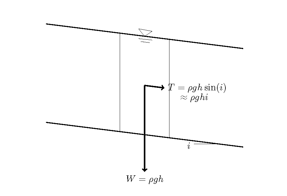
Figure 8.34 : Definition of the shear stress
When we assume that the “shear stress” at that time is \(\tau_0\) , \(\tau_0\) is shear stress of \(T\) per unit area. Then, we have…
In general, the correct way to express the water depth \(h\) in Equation (8.8) is to use the hydraulic radius, \(R\). However, in the case of a channel with a wide rectangular cross section or in the case of 2D calculation, \(h\) is used as is to represent the water depth in each cell.
When the flow is not uniform flow (e.g., non-uniform or undefined flow), then, in (8.8), the shear stress is calculated by using the energy gradient \(I_e\) instead of by using \(i\). Therefore, when applying Manning’s law to 1D flow, the shear stress is expressed as follows.
Where, \(n_m\) is the Manning’s roughness coefficient, and \(<u>\) is the depth-averaged velocity. When the riverbed is composed of uniform material, then the non-dimensional value of \(\tau_0\), which is made dimensionless by the following equation, is called the “non-dimensional shear stress”, or the “Shields number”. This important parameter is frequently used in sediment hydraulics.
Where, \(s\) is the specific gravity of sand particles in water and \(d\) is the grain diameter of the sand. The shear stress, expressed in the dimension of flow velocity as in the following equation, is called the friction velocity and is usually denoted by \(u_*\).
Therefore, the shear stress, \(\tau_0\), is expressed as follows.
Frictional velocity is often understood to be a kind of flow velocity because of its name. However, it is not the flow velocity. It means “the shear stress is expressed in the same dimension as the velocity”.
8.8. Sediment transport type
Sediment transported in rivers can be classified as bed material load (material in the flow that is transported while being exchanged with bed material), and wash load (material that flows downstreamward without being exchanged with bed material). The component of the bed material load, that is transported by rolling, sliding, or jumping near the bed is called the bedload, and the component transported in flowing water under the influence of diffusion by turbulence is called the suspended sediment. In this text, for bed material load, we deal mainly the bedload and the suspended sediment.
8.9. Threshold of bedload motion
Assuming that a sediment particle starts to move when the shear stress \(\tau_0\) or friction velocity \(u_\ast\) exceeds critical values on the riverbed, the critical values are called the thresholds of sediment motion, and the critical values are called the critical shear stress, \(\tau_c\), and the critical friction velocity, \(u_{\ast c}\), respectively. Therefore, whether the riverbed sediment particles are moving or not can be expressed by using \(\tau_c\) or \(u_{\ast c}\), as follows.
The critical shear stress is also expressed in the following dimensionless form, in the same way as the shear stress, and it is called the non-dimensional critical shear stress.
The above equation expresses the \(\tau_c\) used in (8.2) of the previous section.
Iwagaki’s Equation [Ref:5] is often used to express the critical friction velocity of bed materials with a uniform diameter as follows.
Where, \(d\) is the grain diameter whose unit is cm and the unit of \(u_{\ast c}\) is cm/s.
8.10. Suspending and settling velocities of suspended sediments, and possible regions of their existences
In line with the critical bedload for bedload, an important concept for suspended sediment is critical suspension, which involves whether or not sediment can suspend. The critical suspension is determined by the relationship between the magnitude of the suspending velocity and the magnitude of the settling velocity for sediment particles. The following Rubey’s Equation [Ref:6] is the representative equation to express the settling velocity.
Meanwhile, it is said that the moving velocity of sand particles is proportional to the friction velocity. Assuming that \(u_s\) is the moving velocity, their relationship is as follows.
Sand particles in turbulent flow move both horizontally and vertically.
Assuming these relationships, then the critical suspension is…
Consequently,
Using this to classify the regions in which bedload and suspended sediment occur, we obtain the following equation.
Note that the presence of bedload must satisfy the moving conditions given by Equation (8.21) as well as by Equation (8.13). Therefore, it is possible to use these conditions to judge the state of sediment transport in flow over a movable bed.
8.11. Bedload transport formula
The equation that expresses sediment transport when there are sufficient bed materials and when the movement of the bed particles has reached equilibrium is the “equilibrium bedload formula” or simply the “bedload formula” Historically, many bedload transport formulas have been proposed. Here, I introduce representative formulas that are often used.
8.11.1. The Meyer-Peter and Muller (MPM) Equation
The Meyer-Peter and Muller (MPM) Equation [Ref:7] has been frequently used for bed deformation calculations because of its simple form and relatively high adaptability. It is one of the classical hydraulic equations.
Where, \(q_b\) is the unit width bedload transport rate.
8.11.2. Ashida and Michiue Equation
The following Ashida-Michiue Equation [Ref:8], based on more theoretical considerations, is also widely used as an excellent bedload transport equation.
Where, \(\tau_{\ast e}\) is the effective shear stress. It is a dimensionless representation of the shear stress that actually acts on the bed materials and is expressed by the following equation.
Where, \(u_{\ast e}\) is the effective friction velocity. According to Ashida and Michiue [Ref:8], it is expressed by the following equation.
8.12. Suspended sediment
Problems associated with the presence of suspended sediment in river flow tend to very complex. Here, I briefly describe the essential, minimum knowledge required for one to incorporate suspended sediment into riverbed deformation calculations.
8.12.1. Definition of suspended sediment, and the suspended sediment volume.
The suspended sediment concentration \(c\) in flowing water is expressed as the volume of suspended solids per unit volume of flowing water, using the following equation.
Where, \(V\) is the unit volume of fluid (=1), and \(V_s\) is the volume of suspended solid per unit volume of fluid. Consequently, the suspended sediment concentration is dimensionless because it is given by the “volume” divided by “volume”.
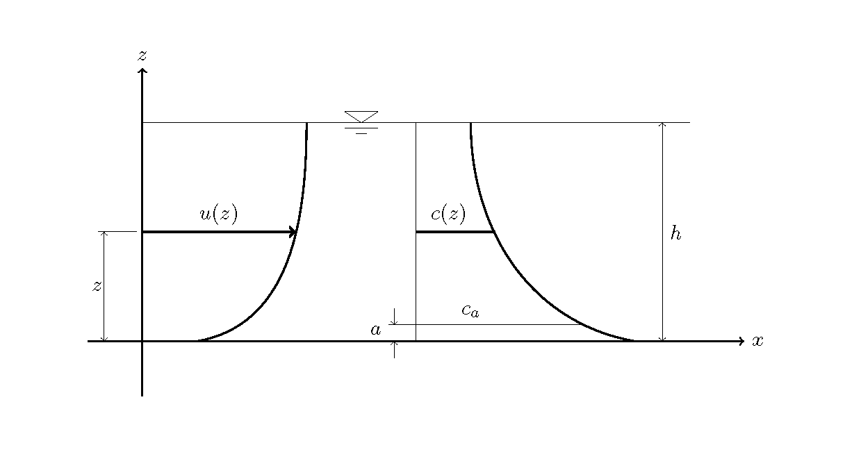
Figure 8.35 : The velocity distribution and the concentration distribution
Assuming a vertical 2D flow, such as Figure 8.35, when the vertical concentration distribution \(c(z)\) and the vertical velocity distribution \(u(z)\) are given, suspended sediment \(q_s\) per unit width can be obtained by the following equation. Refer to [Velocity distribution] for the vertical velocity distribution.
Where, \(h\) is the water depth, \(c(z)\) and \(u(z)\) are the suspended sediment concentration and flow velocity at the height of \(z\) above the bed, respectively, and \(a\) is the height from the bed for the reference point of the concentration.
However, in the 1D and 2D calculations covered in this text, both the velocity and the suspended sediment concentration are calculated using depth-averaged values, so that, for example, in the 2D calculations, \(q_s\) is given by approximation using the following equation.
Where, \(<c>\) is the depth-averaged suspended sediment concentration and \(u\) is the depth-averaged velocity. \(<c>\) is obtained by the 2D advection diffusion equation for 2D channel shape calculation.
In the case of 1D calculations, suspended sediment is not calculated per unit width. Instead, the average suspended sediment is calculated over the entire cross-section using the following equation.
Where, \(<c>\) is the cross-section average concentration and \(Q\) is the discharge.
When calculating riverbed deformation, regardless of whether the calculation is for 1D or 2D, the difference between entrained suspended sediment at (or near) the riverbed and the settled suspended sediment is more important than the suspended sediment itself, as shown in Figure 8.36. This is because the bed deformation is determined by the difference between them.
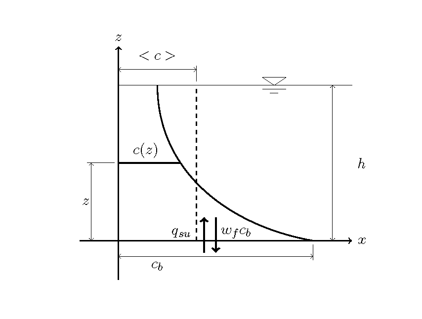
Figure 8.36 :Entrained suspended sediment and settled suspended sediment
Here, settled suspended sediment is expressed by multiplying the settling velocity with the suspended sediment consecration near the bed (= \(w_f c_b\)). \(c_b\) is obtained from the depth-averaged concentration \(<c>\) at the location by a numerical calculation using an equation for the vertical distribution of concentration. The suspended sediment is calculated from the shear stress of calculation point and is expressed as entrained suspended sediment (= \(q_{su}\)). Thus, the changes in riverbed elevation are calculated as the difference between entrained suspended sediment, as calculated based on the shear stress at the location, and settled suspended sediment, as calculated by the space-time distribution. Following is an example for the calculation of sediment concentration distribution in the vertical direction and entrained suspended sediment.
8.12.1.1. Suspended sediment concentration at a reference point and the equation for entrained suspended sediment
entrained suspended sediment is given by following equation.
Where, \(q_{su}\) is entrained suspended sediment per unit area of the bed. It is obtained from the shear stress at the location as described above by assuming a local equilibrium state, while \(c_a\) is the concentration of suspended sediment in the equilibrium-state that corresponds to entrained suspended sediment in the equilibrium state. Although various formulas have been proposed for calculating the suspended sediment concentration at a reference point, \(c_a\) (for example, [Ref:9]), here we introduce the equation proposed by Itakura and Kishi. ([Ref:10])
Where, \(K=0.008\), \(\alpha_\ast=0.14\), \(\rho_s\) is the density of sand particles, and \(\Omega\) is
Where, \(\eta_0=0.5\), \(B_\ast=0.143\) and \(a'=\cfrac{B_\ast}{\tau_\ast}-\cfrac{1}{\eta_0}\). The Itakura and Kishi [Ref:10] equation sets the height of the reference point as \(a=0.05h\).
When the suspended sediment concentration at a reference point, \(c_a\), is given, then under the equilibrium state (i.e., when entrained suspended sediment is equal to settled suspended sediment), entrained suspended sediment can be calculated using the Equation (8.30). When (8.30) is made dimensionless by dividing it by \(\sqrt{sgd}\), the non-dimensional entrained suspended sediment is given by the following equation.
As shown in (8.32), because \(\Omega\) in Formula (8.33) is complicated, the calculation of the formula is also complicated. However, the use of an approximate formula, [Ref:11], makes the calculation simpler than not using such approximate formula. The formula for entrained suspended sediment proposed by Itakura and Kishi [Ref:10] can be approximated by the following equation.
8.12.2. Formula for the suspended sediment concentration distribution and the depth-averaged suspended sediment concentration
The diffusion equation for suspended sediment concentration in the depth direction under steady flow conditions is given by
Where, \(\epsilon\) is the diffusion coefficient of suspended sediment in the depth direction. Assuming that the settling velocity \(w_f\) is constant in the depth direction, we integrate (8.35) with respect to \(z\). Considering the conditions under which no particles are ejected from the water surface, we derive the following formula.
First, assuming that \(\epsilon\) is constant in the depth direction, we integrate Formula (8.36) with respect to \(z\). Next, we assume that the suspended sediment concentration at the riverbed (\(z=0\)) is \(c_b\). Then, we derive the following formula for the suspended sediment concentration distribution.
Where, \(\beta=\cfrac{w_f h}{\epsilon}\) and \(\zeta=z/h\).
- Equation (8.37) is an exponential distribution equation and is called the Lane and Kalinske Equation [Ref:12].
Integrating this equation again from 0 to 1 with respect to \(\zeta\) yields the depth-averaged concentration, \(<c>\).
In the 1D and 2D riverbed deformation calculations described later, concentrations of suspended sediment are basically calculated as depth-averaged values, \(<c>\). However, because bed deformation needs to be discussed in relation to the suspended sediment concentration at the bottom of flow, which is in contact with the bed, an equation that relates the depth-averaged concentration to the near-bed concentration is required. Equation (8.38) is used for this purpose.