6. The 2D advection equation

6.1. Basic formulas

Here I show the 2-dimensional advection equation.

(6.1)\[{{\partial f}\over{\partial t}} + u{{\partial f}\over{\partial x}}+ v{{\partial f}\over{\partial y}} = 0\]

Where, \(t\) is the time, \(x, y\) are the axes of Cartesian coordinates, \(f\) is a variable to be advected, and \(u,v\) are advection velocities in the directions of \(x, y\).

Similar to the 1D advection equation, while the distribution form is maintained, the theoretical solutions to this equation, \(f\), move in the direction of \(x\) at a velocity of \(u\) and in the direction of \(ｙ\) at a velocity of \(v\).

6.2. The upwind difference scheme

The upwind difference equation for the advection term is as follows.

(6.2)\[\begin{split}u>0 \mbox{When}; \; \; u\cfrac{\partial f}{\partial x}=u\cfrac {f(i,j)-f(i-1,j)}{\Delta x} \\ u<0 \mbox{When}; \; \; u\cfrac{\partial f}{\partial x}=u\cfrac {f(i+1,j)-f(i,j)}{\Delta x}\end{split}\]

(6.3)\[\begin{split}v>0 \mbox{When}; \; \; v\cfrac{\partial f}{\partial x}=v\cfrac {f(i,j)-f(i,j-1)}{\Delta y} \\ v<0 \mbox{When}; \; \; v\cfrac{\partial f}{\partial x}=v\cfrac {f(i,j+1)-f(i,j)}{\Delta y}\end{split}\]

Where, \(\Delta x, \Delta y, \Delta t\) are the calculation step sizes in the directions of \(x, y, t\), respectively, and \((i,j)\) are the grid numbers in the directions of \((x,y)\), respectively. Consequently, for example, when \(u>0, \; v>0\), the difference scheme for Equation (6.1) is as follows.

(6.4)\[\cfrac{f_n(i,j)-f(i,j)}{\Delta t}+ u\cfrac{f(i,j)-f(i-1,j)}{\Delta x}+ v\cfrac{f(i,j)-f(i,j-1)}{\Delta y}=0\]

Where, \(f_n(i,j)\) is the value of \(f(i,j)\) at \(t=t+\Delta t\). From Equation (6.4), \(f_n(i,j)\) can be obtained by repeating calculations for the following equation for a step of \(\Delta t\). In this case, the scheme gives a backward difference in the direction of \(x\) and in the direction of \(y\).

(6.5)\[f_n(i,j)=f(i,j)-\Delta t \left\{ u\cfrac{f(i,j)-f(i-1,j)}{\Delta x}+ v\cfrac{f(i,j)-f(i,j-1)}{\Delta y}\right\}\]

6.2.1. An example of calculations by backward difference scheme

This is an example of calculation for when \(u>0, \; v>0\). The initial distribution of \(f\) is conical, as shown in Figure Figure 6.1.

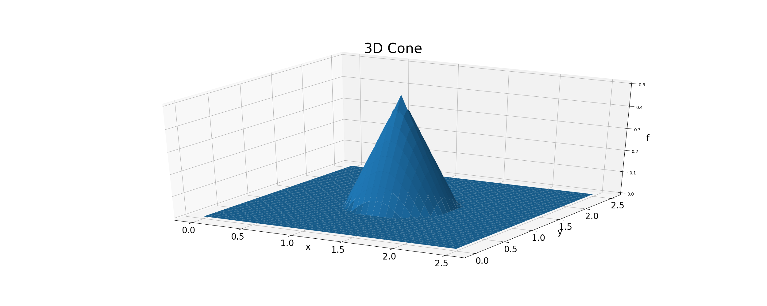
Figure 6.1 : Initial conditions for the 2D advection calculations

A conical distribution is given by following equation.

(6.6)\[\begin{split}r<R \; \mbox{When;} & f(x,y)=\cfrac{R-r}{R} f_p \\ r>R \; \mbox{When;} & f(x,y)=0\end{split}\]

Where,

(6.7)\[r=\sqrt{(X_p-x)^2+(Y_p-y)^2}\]

Where, \(X_p, Y_p\) are the locations of peaks, \(f_p\) is the value of the peak, and \(R\) is the radius of the bottom.

6.2.1.1. The Python code and a calculation example

The Python code using (6.5) is as follows. https://github.com/YasuShimizu/Python-Code/blob/main/2d_backward_p3d.py The following figure shows the calculation results calculated by using the code. In this example, \(u=v=0.5\) (m/s) and:math:f_p=0.5, R=20 (m).

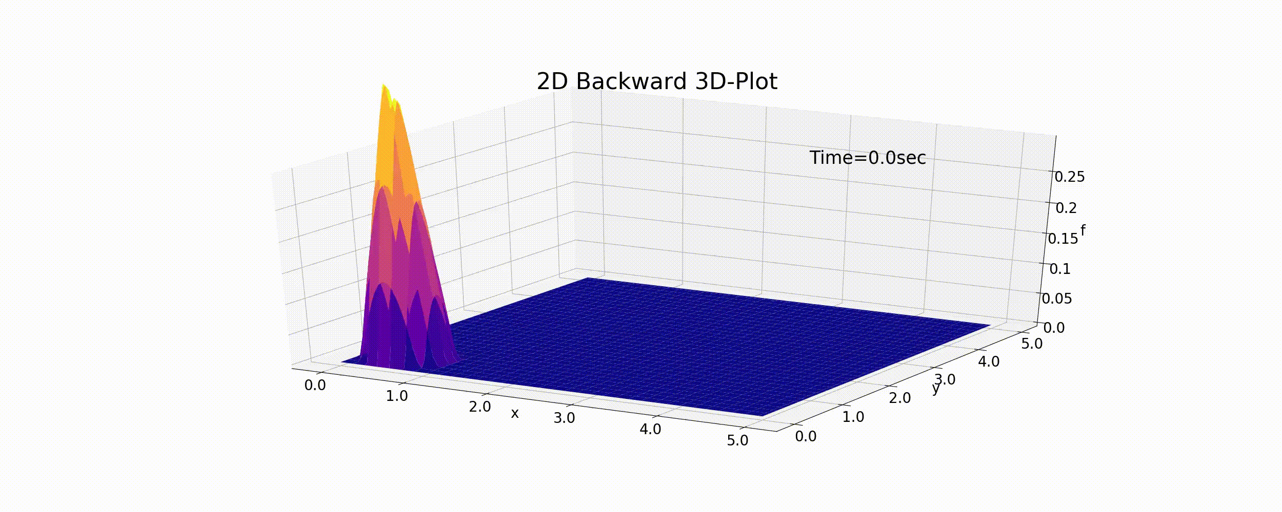
Figure 6.2 : The calculation results for the 2D advection equation (backward difference scheme)

As with the 1D case, the peak values gradually decrease due to numerical diffusion and the cone gradually flattens while it moves. The results of this calculation are not entirely accurate.

6.2.2. The upwind difference scheme with varying advection direction

The updating formula for \(f\) in which the advection terms of Equation (6.2) and Equation (6.3) are expressed with one equation is as follows.

\[f_n(i,j)=f(i,j)\]

\[-\cfrac{\Delta t}{2 \Delta x} \left[(u+|u|)\left\{f(i,j)-f(i-1,j)\right\}+(u-|u|)\left\{f(i+1,j)-f(i,j)\right\} \right.\]

(6.8)\[+\left.(v+|v|)\left\{f(i,j)-f(i,j-1)\right\}+(v-|v|)\left\{f(i,j+1)-f(i,j)\right\} \right]\]

Equation (6.8) is an upwind difference scheme that can be applied regardless of the sizes or signs of of \(u, v\).

Now, let us try to test this 2D upwind difference scheme under the condition where \(u, v\) vary. We assume that \(u,v\) is expressed by the following equations.

(6.9)\[\begin{split}u = & -r_t \omega \sin \theta \\ v = & r_t \omega \cos \theta\end{split}\]

The motion expressed by these equations is circular, where \(r_t\) is the radius of curvature for circular motion, \(\omega\) is the angular velocity, and \(\theta\) is the phase angle. Assuming that the peak of the cone shown in Figure Figure 6.1 moves according to Equation (6.9), the calculation results are shown by the following figure (Figure 6.3). In this example, \(T\) is the period of circular motion, and when we assume that \(T=\) = 100 sec, \(r_t\) = 30 m and f_p = 0.5. The relationship between \(T\) and \(\omega\) is given by the following equation.

(6.10)\[\omega=\cfrac{2\pi}{T}\]

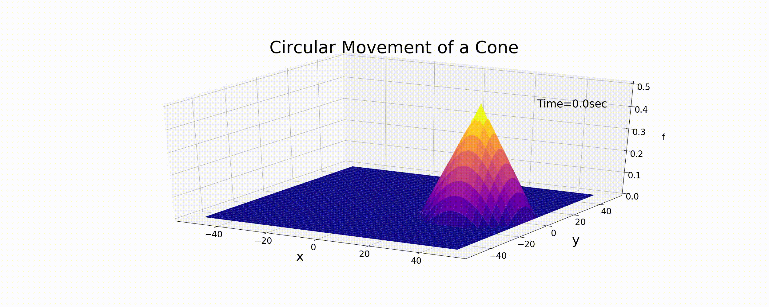
Figure 6.3 : Circular motions of the cone

Figure 6.3 is given merely by moving the distribution of the cone with the velocity of Equation (6.9). It is not the difference calculation　result for Equation (6.1). However, in a sense, this is the target exact solution for the numerical calculations we will be performing. For reference, the Python code for calculating the animation of Figure 6.3 is below.

https://github.com/YasuShimizu/Python-Code/blob/main/3dcone_circle_m3d.py

I am sorry for the long introduction, but now let us try the upwind difference scheme of the 2D advection equation, which is the goal of this section.

6.2.2.1. The Python code and a calculation example

Below is the Python code using Equation (6.1).

https://github.com/YasuShimizu/Python-Code/blob/main/2d_upwind_circle.py

Using this code, under the initial conditions of Equation (6.6), \(u,v\) are varied using Equation (6.9). The results are shown in the figure below.

Figure 6.4 : Calculating the circular motion for a conical distribution by using the 2D upwind difference scheme

As expected, the upwind difference scheme results in the gradual diffusion of the initial shape and in the attenuation of the peak values. Although the calculation results are stable, as they were the 1D calculation, the upwind difference scheme is proven not to give accurate calculation results.

6.2.2.2. Problem (4)

\(f\) is a variable whose initial condition is the cone-shape distribution.

Calculate the changes in \(f\) with time when \(f\) continuously moves along the sides of the rectangular area.

6.3. The higher-order difference scheme

Here, as I explained for the 1D higher-order difference scheme, I describe the 2D version of the CIP method as a 2D higher-order difference scheme.

6.3.1. Calculating the advection term by using the 2D CIP method

To simplify the explanation, first, we calculate for when \(u<0\) and \(v<0\).

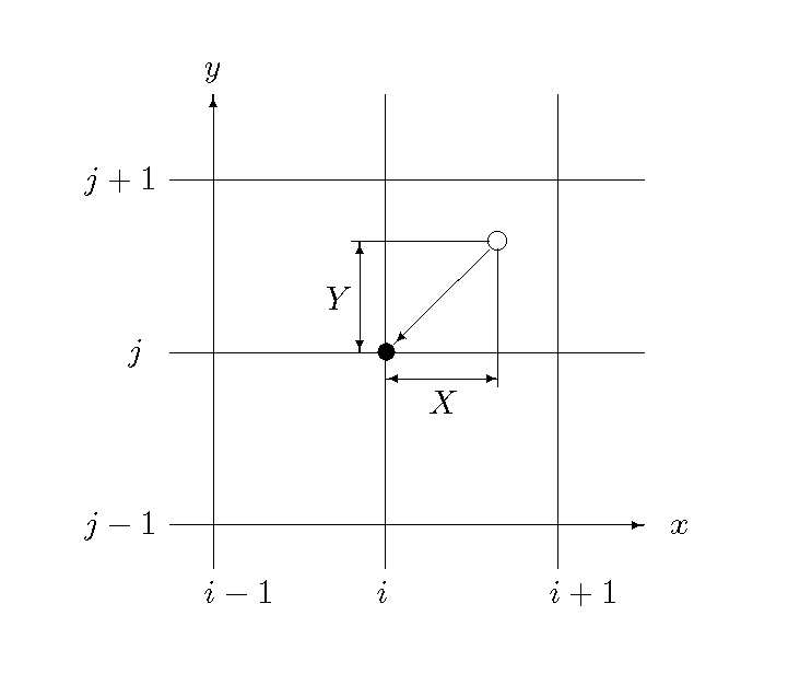
Figure 6.5 : Estimating \(f\) on the calculation plane

As shown in Figure 6.5, set the calculation point numbers in the \(x, y\) directions as \(i,j\). We assume that points within the range of \(i, i+1, j, j+1\) (shown by the white dot) at time \(t\) move during the time of \(\Delta t\) to the black dot in the figure. 前

As was explained for the 1D calculation, this is a problem for the estimation of the distribution of \(f\) regarding the black dot in Figure 6.5. How can we estimate the distribution form of \(f\)? Therefore, assuming that when…

(6.11)\[X=-u \Delta t, \; \; Y=-v \Delta t\]

When we can estimate the distribution form of \(F(X,Y)\), we have…

(6.12)\[f(i,j,t+\Delta t) = F(X, Y)\]

With this, we can update the time of \(f\). Note that, here, \(f\) is a discrete value for the \((i,j)\) grid, and \(F\) is a continuous function.

Although \(F\) was assumed to be a curve of the third order for the 1D problem, here we assume it to be a surface of the third order. \(F(X,Y)\) must satisfy the following relationships when \(X=0, Y=0\).

(6.13)\[F(X,Y)=f(i,j), \; \; \; F_x(X,Y)=f_x(i,j), \; \; \;F_y(X,Y) = f_y(i,j)\]

(Where, \(F_x(X,Y)=\displaystyle{{\partial F}\over{\partial x}}\), \(F_y(X,Y)=\displaystyle{{\partial F}\over{\partial y}} (X,Y)\), \(f_x(i,j)=\displaystyle{{\partial f}\over{\partial x}} (i,j)\), \(f_y(i,j)=\displaystyle{{\partial f}\over{\partial y}} (i,j)\).)

Therefore, we set \(F(X,Y)\) as follows.

(6.14)\[\begin{split}F(X,Y) = \left[ (a_1 X + c_1 Y + e_1) X + g_1 Y + f_x(i,j) \right] X + \\ \left[ (b_1 Y + d_1 X + f_1) Y + f_y(i,j) \right] Y + f(i,j)\end{split}\]

This equation automatically satisfies Equation (6.13). Other conditions that need to be satisfied are…

(6.15)\[\begin{split}F(0,-\Delta y)=f(i,j+1), \; \; \; F(-\Delta x, 0)=f(i+1,j) \\ F(-\Delta x, -\Delta y) = f(i+1,j+1), \; \; \; F_x(0, -\Delta y)=f_x(i,j+1) \\ F_x(-\Delta x, 0)=f_x(i+1,j), \; \; \; F_x(-\Delta x, -\Delta y) = f_x(i+1,j+1) \\ F_y(0, -\Delta y)=f_y(i,j+1), \; \; \; F_y(-\Delta x, 0)=f_y(i+1,j)\end{split}\]

By using these relationships, the factors in Equation (6.14) are as follows.

\[a_1 = {{ \left[ f_x(i+1,j)+f_x(i,j) \right] \Delta x +2 \left[ f(i,j)-f(i+1,j) \right]}\over{\Delta x^3}}\]

\[b_1 = {{ \left[ f_y(i,j+1)+f_y(i,j) \right] \Delta y +2 \left[ f(i,j)-f(i,j+1) \right]}\over{\Delta y^3}}\]

\[c_1 = {{-\left\{ f(i,j)-f(i,j+1)-f(i+1,j)+f(i+1,j+1)\right\}-\left[f_x(i,j+1)-f_x(i,j) \right] \Delta x }\over{\Delta x^2 \Delta y}}\]

\[d_1 = {{-\left\{f(i,j)-f(i,j+1)-f(i+1,j)+f(i+1,j+1)\right\}- \left[ f_y(i+1,j)-f_y(i,j) \right] \Delta y}\over{\Delta x \Delta y^2}}\]

\[e_1 = {{ 3 \left[ f(i+1,j)-f(i,j) \right] + \left[ f_x(i+1,j)+2 f_x(i,j) \right] \Delta x }\over{\Delta x^2}}\]

\[f_1 = {{ 3 \left[ f(i,j+1)-f(i,j) \right] + \left[ f_y(i,j+1)+2 f_y(i,j) \right] \Delta y }\over{\Delta y^2}}\]

(6.16)\[g_1 = {{-\left\{f_y(i+1,j)-f_y(i,j)\right\}+c_1 \Delta x^2 }\over{\Delta x}}\]

6.3.1.1. Problem (5)

Derive Equation (6.16) to check whether the expression of \(a_1 \sim g_1\) is right.

6.3.2. Calculating the advection term with the 2D CIP method (generalization)

The explanation thus far is for \(u<0\) and \(v<0\). Actually, there are eight possible combinations for the combinations of signs of \(u, v\). However, it would be very complicated to formulate and program all the combinations. Therefore, we introduce a sign function (\(\mbox{sign}\)) as we did for the ID calculation.

(6.17)\[\begin{split}i_s = \mbox{sign}(u), \; \; \; & j_s = \mbox{sign}(v) \\ i_m = i-i_s, \; \; \; & j_m = j-j_s\end{split}\]

\(F(X,Y)\), the distribution form of the variables between grids, is defined as (6.18) by defining \(X, Y\) as Figure 6.6, and by transforming Equation (3.7) to the second order.

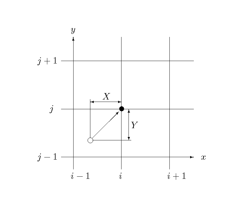
Figure 6.6 : Defining \(X, Y\) on the calculation plane

(6.18)\[\begin{split}F(X,Y) = \left[ (a_1 X + c_1 Y + e_1) X + g_1 Y + f_x(i,j) \right] X + \\ \left[ (b_1 Y + d_1 X + f_1) Y + f_y(i,j) \right] Y + f(i,j)\end{split}\]

Where, the factors \(a_1 \sim g_1\) are expressed as follows by using \(i_s, j_s, i_m, j_m\), regardless of the signs of \(u, v\).

\[a_1 = {{ i_s \left[ f_x(i_m,j)+f_x(i,j) \right] \Delta x -2 \left[ f(i,j)-f(i_m,j) \right]}\over{i_s \Delta x^3}}\]

\[b_1 = {{ j_s \left[ f_y(i,j_m)+f_y(i,j) \right] \Delta y -2 \left[ f(i,j)-f(i,j_m) \right]}\over{j_s \Delta y^3}}\]

\[c_1 = {{ -\left\{f(i,j)-f(i,j_m)-f(i_m,j)+f(i_m,j_m)\right\}-i_s \left[f_x(i,j_m)-f_x(i,j) \right] \Delta x }\over{j_s \Delta x^2 \Delta y}}\]

\[d_1 = {{ -\left\{f(i,j)-f(i,j_m)-f(i_m,j)+f(i_m,j_m)\right\}- j_s \left[ f_y(i_m,j)-f_y(i,j) \right] \Delta y}\over{i_s \Delta x \Delta y^2}}\]

\[e_1 = {{ 3 \left[ f(i_m,j)-f(i,j) \right] + i_s \left[ f_x(i_m,j)+2 f_x(i,j) \right] \Delta x }\over{\Delta x^2}}\]

\[f_1 = {{ 3 \left[ f(i,j_m)-f(i,j) \right] + j_s \left[ f_y(i,j_m)+2 f_y(i,j) \right] \Delta y }\over{\Delta y^2}}\]

(6.19)\[g_1 = {{-\left\{f_y(i_m,j)-f_y(i,j)\right\}+c_1 \Delta x^2 }\over{i_s \Delta x}}\]

6.3.2.1. Problem (6)

Derive Equation (6.19) to check whether the expression of \(a_1 \sim g_1\) is right.

6.3.3. Updating the differentiation amount

Under the CIP method, in addition to the variable \(f\), its differentiation, \(f_x, f_y\), also needs to be updated from time to time. Now, we perform partial differentiation for both sides of Equation (6.1) with respect to \(x\).

(6.20)\[{{\partial^2 f}\over{\partial t \partial x}} + {{\partial u}\over{\partial x}} {{\partial f}\over{\partial x}} + u {{\partial^2 f}\over{\partial x^2}} + {{\partial v}\over{\partial x}} {{\partial f}\over{\partial y}} + v {{\partial^2 f}\over{\partial x \partial x}} =0\]

Assuming that \(\displaystyle{{{\partial f}\over{\partial x}}}\) is \(f_x\), we have…

(6.21)\[{{\partial f_x}\over{\partial t}} + u{{\partial f_x}\over{\partial x}} + v{{\partial f_x}\over{\partial y}} = -\left( f_x {{\partial u}\over{\partial x}} + f_y {{\partial v}\over{\partial x}} \right)\]

As we can see, the left side is a 2D advection equation with respect to :f_x. This means that, here, we can directly apply the 2D CIP method. When \(u, v\) are constants, the right side is 0. When they are variables, we can apply [ The basic concept of the CIP method ], which is explained under the 1D CIP method. The calculation should apply the split method. The central difference scheme can be applied for the difference form on the right side.

Similarly, when we perform partial differentiation for Equation (6.1) with respect to \(y\), and we assume that \(\displaystyle{{{\partial f}\over{\partial y}}}\) is \(f_y\), then we have…

(6.22)\[{{\partial f_y}\over{\partial t}} + u{{\partial f_y}\over{\partial x}} + v{{\partial f_y}\over{\partial y}} = -\left( f_x {{\partial u}\over{\partial y}} + f_y {{\partial v}\over{\partial y}} \right)\]

This is the same form as Equation (6.21). Therefore, the advection term on the left side can be calculated with the CIP method, and the source term on the right side can be calculated with a central difference scheme.

6.3.4. The Python code and a calculation example

The Python code for the 2D CIP method mentioned above is found at…

https://github.com/YasuShimizu/2d_advection_cip

The calculation that results from the code is shown below. The calculation conditions are the same as the aforementioned The upwind difference scheme; that is, a cone distribution with circular motion.

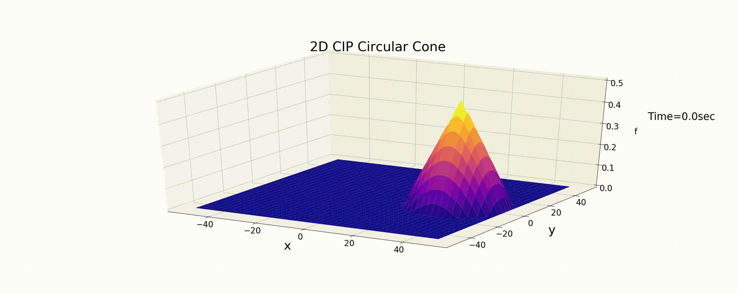
Figure 6.7 : The calculation results for the 2D advection equation (the CIP method)

The calculation results show that the circular motion continues and that the cone shape is largely preserved. The CIP method is a numerical calculation method for the 2D advection equation and gives highly accurate calculation results.