14. Calculations of 2D flow and bed deformation in a channel with width variation
14.1. Equation of continuity
When the river width changes in the downstream direction, the equation of continuity can be approximated by the following equation, instead of by Equation (11.4).
Where,
Similarly, in Equation (13.20), because \(\Delta n\) changes according to the changes in river width, Equation (13.20) can be used without any modifications for as the equation of continuity of sediment transport.
14.2. A calculation example for a widened channel
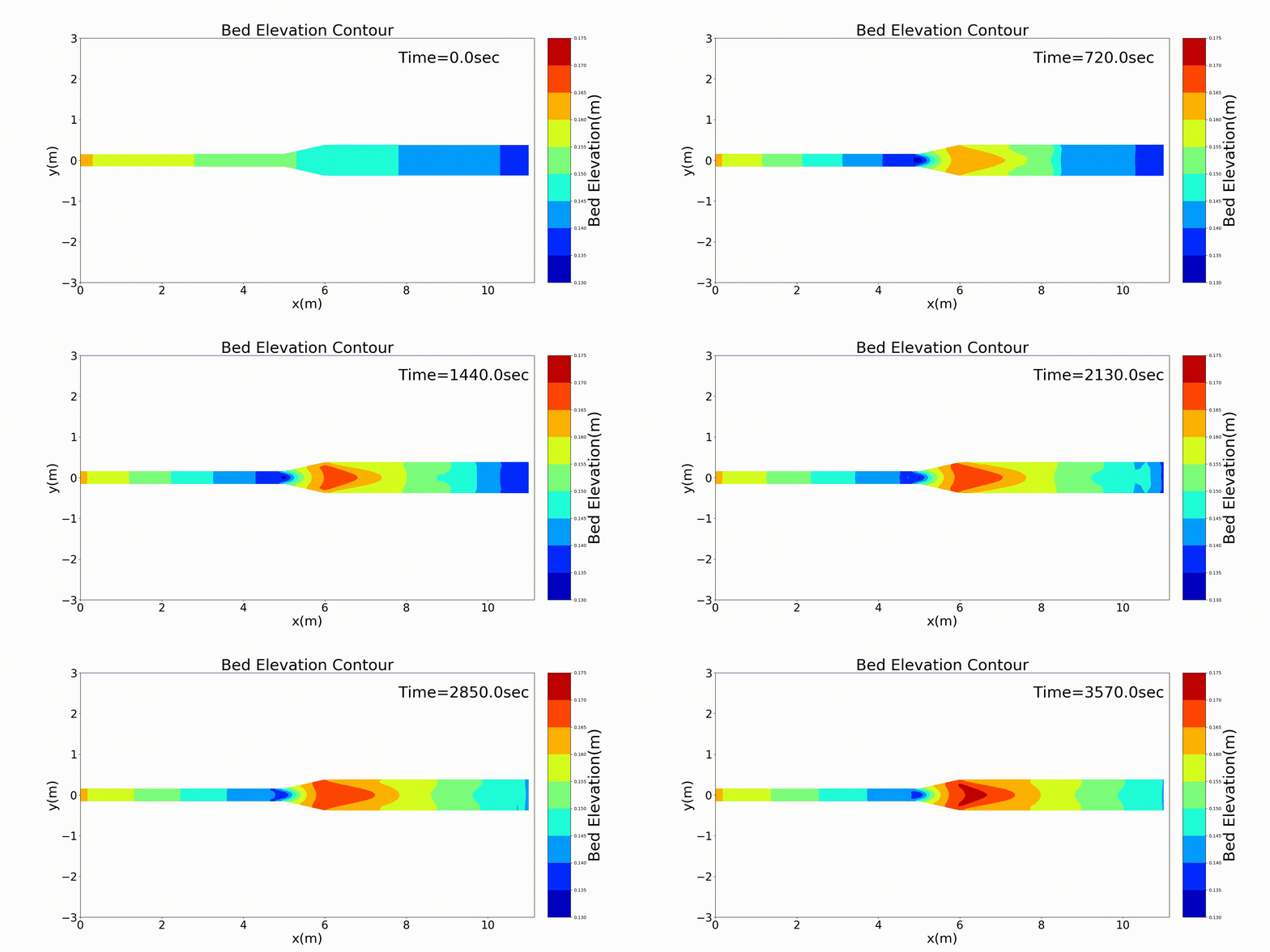
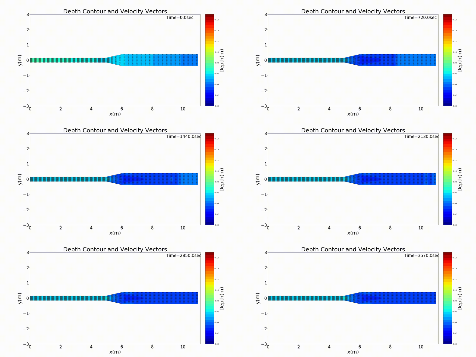
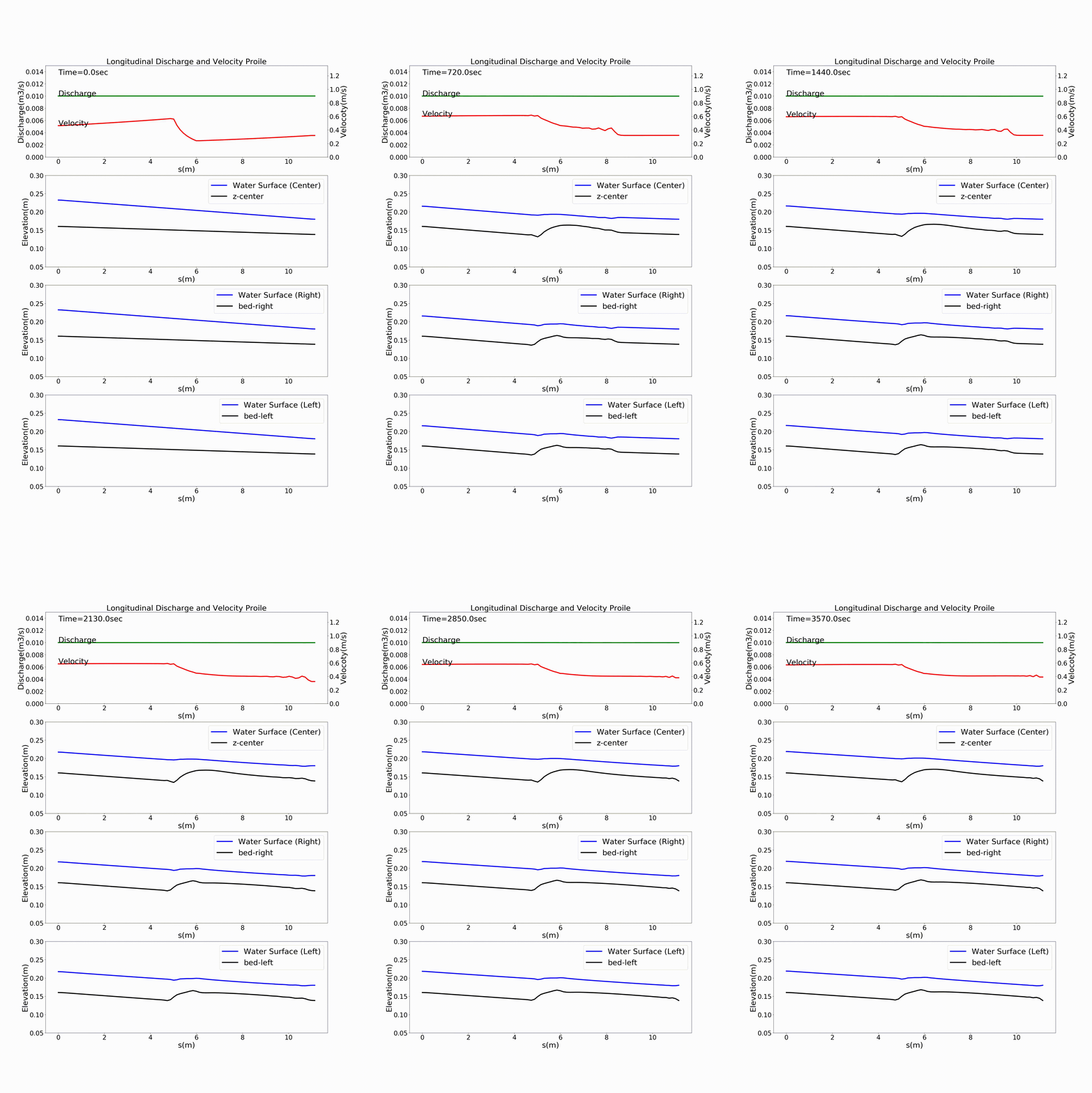
As a typical example of a channel that varies in width in the downstream direction, here is an example of a calculation for a channel that has a rapidly widening section. For a channel with a bed gradient of \(i=1/500\) and with a channel width 30 cm in the upstream section that sharply triples in width to 90 cm around the midpoint of the channel, a bed material with a uniform grain size of \(d=\) =1.35 mm is placed and a constant discharge of \(Q=\) 10 L/s is given. The following example shows the results for flow and bed deformation calculations for this channel. Figure 14.1 shows the temporal changes in the bed elevation, Figure 14.2 shows the water depth and the vector of depth-averaged velocity, and Figure 14.3 shows the longitudinal distributions of the discharge and the velocity as well as the water depth and the bed elevation.

Figure 14.1 : Calculation results for bed deformation in a rapidly widening channel

Figure 14.2 : Calculation results of changes in the velocity vector and the water depth in a rapidly widening channel

Figure 14.3 : Longitudinal distributions of discharge and velocity, and longitudinal profiles of the water level and the bed elevation along the channel center line, the left bank, and the right bank in a rapidly widening channel
14.3. The Python code
The Python code used in the above example for calculating 2D flow and bed deformation for a river with a changing width is as follows.
https://github.com/YasuShimizu/2d_width_variation
By launching “run.py” in this file, the above example calculations are automatically performed, plotted, and animated. Three folders – bed, png, and png_q – must be created under the execution folder. In these folders, image files are generated for each calculation time step, and an animation is finally generated from the image files. The calculation conditions are all described in the file [Case1.yml] shown below. By changing the parameters as necessary, calculations can be performed under different conditions.
j_param: 1 # channel shape data input method (1=constant gradient, 2=data input)
# when j_param=1
slope: 0.002 # overall gradient
eta_upe: 0.1606 # bed elevation at the upstream end when gradient data is given
# when j_param=2
bed_file: Q10_xzb.csv
j_rep: 0 # periodic boundary conditions (0: no periodic boundary conditions, 1: periodic boundary conditions)

lam : 11 # channel wavelength (m)
nx0 : 80 # number of girds/wavelength
ny : 15 # number of girds in the transverse direction (Use an odd number is recommended)
wn : 1 # wave number
chb : 0.3 # channel width (m)
t0_degree : 0 # max. mender deflection angle (degree)

j_exp: 1 # 0=no change in the width, 1=change in the width
xb1: 5 # width change point
xb2: 6
xb3: 10
br0: 1.0 # width change rate
br1: 1.0
br2: 2.5
br3: 2.5
br4: 2.5

xsize: 20 # transverse scale of the figure for plotting the calculation results


amp : 0.0 # wave height of the initial bed bar (m)
delta : 0. # phase difference of the initial bed bar(m)
beta_0: 0. # rate of channel narrowing at the inner bank
amp_0: 0.0 # bed elevation of the narrowed section (m)

snu_0 : 1e-6 # coefficient of kinematic viscosity
hmin : 0.0001 # min. water depth (m)
vmin : 0.0001 # min. water velocity (m)
cw: 0.001 # sidewall friction coefficient
ep_alpha: 1. # eddy viscosity coefficient

qp: 0.01 # discharge (m^3/s)
snm: 0.0167 # Manning’s roughness coefficient
g: 9.8 # gravitational acceleration (m/s^2)
diam: 0.00135 # average grain diameter of bed materials (m)
slambda: 0.4 # void ratio
musk: 0.2 # μs × μk “static friction coefficient” × “dynamic friction coefficient”
nsta: 7.0 # secondary flow intensity

j_west: 0 # upstream condition (0: open, 1: closed)
j_east: 0 # downstream condition (0: open, 1: closed)
j_hdown: 1 # water level condition at the downstream end (0: free flow, 1: neutral depth, 2: constant water level)
h_down : 1. # constant water level when j_hdown=2 (m)
j_inih: 0 # initial longitudinal water surface profile (0: straight, 1: uniform flow calculation, 2: non-uniform flow calculation)

alh: 0.7 # relaxation factor for the water level convergence calculation
lmax: 10 # max. number of repetitions of the water level convergence calculation at each time step

etime: 3600. # calculation end time (sec)
tuk: 30. # output interval of calculation results (sec)
dt: 0.005 # calculation time step (sec)
stime: 0. # output start time (sec)
bstime: 20. # bed deformation start time (sec)

j_obst: 0 # obstacles (0=No, 1=Yes)
jo_type: 2 # method for installing obstacles (1=read from a file, 2=specify the condition)
jo_method: 4 # 0=No, 1=only right bank, 2=only left bank, 3=right & left banks (alternately), 4=right & left banks (at the same longitudinal locations)
f_dike_pos: 0.8 # position of the first spur dike (m)
dike_dis: 0.8 # interval of spur dikes (m)
dike_length: 0.1 # length of spur dike (m)
dike_thick: 0.02 # width of spur dike (m)
num_dike : 3 # number of spur dikes (per bank)

iskip: 2 # i-direction thinning of vector plots
jskip: 1 # j-direction thinning of vector plots
jscale: 30 # flow vector scale factor

alpha_upu : 0.1 # relaxation factor of periodic boundary conditions
rrmax: 1 # max. curvature plot value on an axis (1/m)
z_step: 0.005 # step of bed contour

zhmin: 0.05 # min. longitudinal profiles of bed and water level
zhmax: 0.3  # max. longitudinal profiles of bed and water level