Appendix IV (1D non-uniform flow calculation)
1D non-uniform flow calculation
1D non-uniform flow calculation is a 1D analysis method for open channels with a steady flow field. It is a basic method for calculating the water surface profile of rivers. It is still used today in the calculation of the design high water level of many rivers. In 2D calculations covered in this text, ID non-uniform flow calculation is used as one of the methods for calculating the initial water surface profile by means of iterated calculation.
The equation for 1D flow in a channel with an arbitrary cross-sectional profile (the non-uniform flow equation) is expressed by following equation.
Where, \(H\) is the water level, \(x\) is the distance in the flow direction, \(V\) is the mean sectional velocity, \(g\) is the gravitational acceleration, \(I_e\) is the energy gradient, and \(\alpha_e\) is the energy correction coefficient. Details are omitted here because there are precise explanations in [Ref:37]. \(I_e\) and \(\alpha_e\) are expressed as follows.
Where, \(n_y\) is the number of divisions in the transverse direction, \(n_{mj}\), \(h_j\) and \(u_j\) are the \(j\) th Manning’s roughness coefficient, the water depth and the flow velocity when the cross-section is divided in the transverse direction. The division method is as shown in Figure 14. Also, \(Q\) is discharge, \(A\) is the cross-sectional area, and \(V\) is the mean sectional velocity.
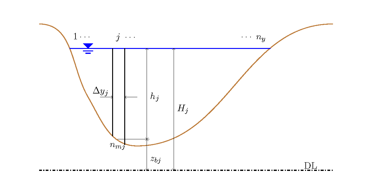
Figure 14 : Division of the cross-section in the transverse direction
From the upstream end to the downstream end of the channel, the distance between the \(i-1\) th cross-section and the \(i\) th cross-section is expressed as \(\Delta x\). And (130) is shown in differences.
In the equation above, \(i\) is on the downstream side and \(i-1\) is on the upstream side. For an ordinary flow, the water surface elevation at the downstream end is given as the boundary condition, and the water surface elevation is obtained by repeating calculation toward \(H_i \rightarrow H_{i-1}\).
In the calculation code of 2D flow in meandering channels [Calculation of 2D flow in meandering channels (practical edition)], this non-uniform flow calculation method is used as one of methods for setting the initial water level distribution.